Introduction
- spark - developed at uc berkley as an improvement of hadoop
- it borrowed concepts from hadoop but now works independent of it
- unlike hive etc, spark doesn’t convert into the map reduce equivalent
- it is much more performant than hadoop
- it offered much more flexibility when compared to hadoop -
- unlike hadoop which relies on yarn as a cluster manager, it can also work with different cluster managers like mesos and kubernetes. cluster manager, resource manager, container orchestrator, etc all mean the same thing
- unlike hadoop which relies on hdfs for storage, it can also work with cassandra, cloud storage options like s3, azure blob storage, etc
- eventually, it became its own thing as it has much more features
- why spark is popular - we write for e.g. sql and all the complexities around distributed processing is abstracted away from us. also, it is a unified platform - all capabilities - including batch processing, stream processing and ml are in one platform
- databricks - founded by original developers of spark. for e.g. it makes deploying spark applications much easier, has an optimized runtime for spark, etc
Databricks Community Edition Basis
- first, create an account - remember to select community edition and not the cloud providers like aws etc
- then, login to your account from here
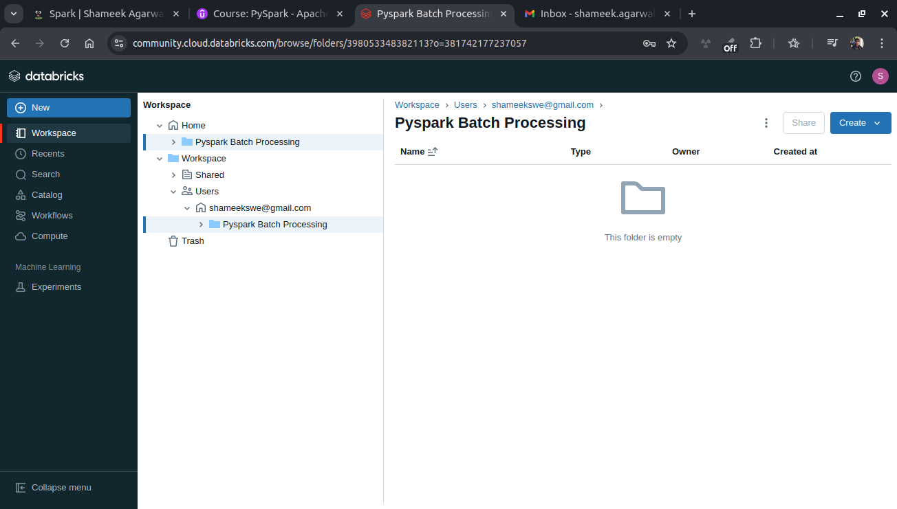
- workspace directories allow us to create multiple directories. by default, we can see the shared and users directory
- we should typically create our project directories under our user in the users directory
![]()
- we can create notebooks inside these project directories
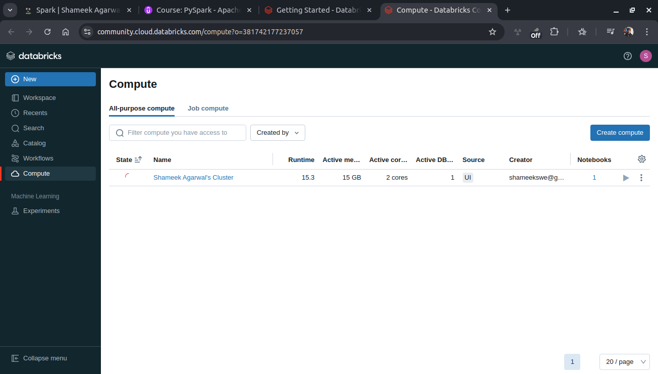
- we can create a free single node cluster in this community edition in the compute tab. aws is used underneath i believe
![]()
- note - clusters are terminated after 1 hr of inactivity. we cannot restart them, we need to create a new cluster
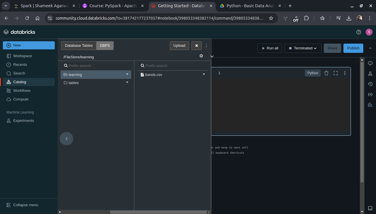
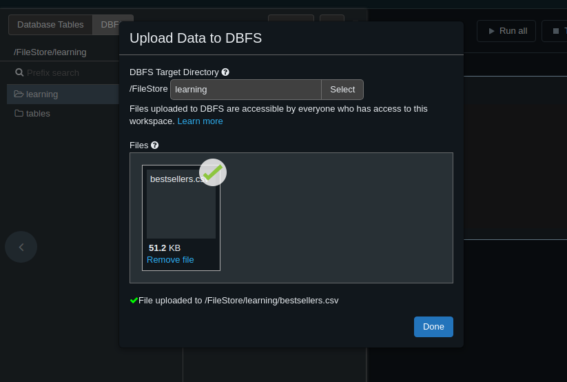
- we also get some free storage. we can access it and upload files to it by going to catalog -> dbfs aws s3 is used underneath i believe
![]()
- we can specify a custom nested directory to upload this file to as well
![]()
- with the code below, we can see the output -
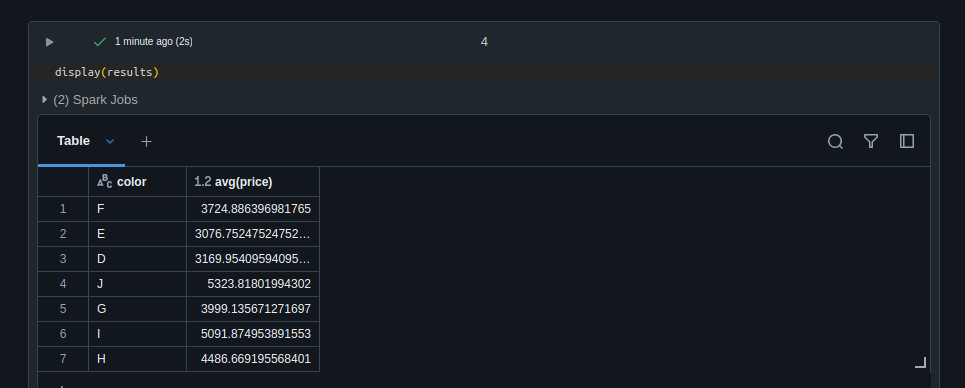
diamonds = (
  spark.read.format("csv")
    .option("header", "true")
    .option("inferSchema", "true")
    .load("/databricks-datasets/Rdatasets/data-001/csv/ggplot2/diamonds.csv")
)

from pyspark.sql.functions import avg

results = (
  diamonds.groupBy('color')
    .agg(avg('price'))
)

results.show()
color avg(price) F 3724.886396981765 E 3076.7524752475247 D 3169.9540959409596 J 5323.81801994302 G 3999.135671271697 I 5091.874953891553 H 4486.669195568401 - we can also use the
displaymethod, which gives a more interactive version of the tabledisplay(results)![]()
Local Environment Setup Basics
- for running via ide, create a virtual environment
- install pyspark
- run the code below simply using ide / python file.py -
from pyspark.sql import * if __name__ == '__main__': spark = ( SparkSession.builder .appName('') .master('local[*]') .getOrCreate() ) people_list = [ {'name': 'david', 'age': 33}, {'name': 'ravi', 'age': 28}, {'name': 'abdul', 'age': 35}, ] people = spark.createDataFrame(people_list) people.show() - we are using the local cluster manager here
- we can also use spark-submit if we have spark downloaded as follows. note that spark-submit too by default uses the local cluster manager -
~/spark-3.5.1-bin-hadoop3/bin/spark-submit ~/Desktop/library/pyspark-batch-processing/dataframe-vs-sql.py - cloud services like google dataproc make it very easy to setup spark running over a hadoop cluster, libraries like zeppelin notebooks, integration with google storage (s3 equivalent of gcp), etc. at that point, we can use these tools like spark-submit, and submit our packaged application. we would slightly modify the shell command above and add
--master yarnto it
For Anaconda
- just had to run
conda install conda-forge::pyspark - now, i am able to use it easily from
jupyter-notebook
Dataframes vs SQL
- spark offers two different ways - using spark databases vs using dataframes
- dataframes are a runtime concept. metadata related to dataframes are stored in catalog, which too only exist during the runtime
- spark databases are stored in file systems like hdfs, s3, etc in formats like csv, json, etc. the metadata related to spark databases is stored inside a metastore, which too is inside a physical storage
- note - i believe that the spark database concept is somewhat built on top of hive
- so, the main difference is while the spark dataframes go away when the application terminates, the spark databases stay in the storage and are visible across applications
- we use plain sql strings to interact with spark databases and tables, while we use api to interact with dataframes
- note that we can inter-convert between the two so that dataframes can be used via sql / spark databases can be accessed via api
- i also think spark databases have features like bucketing and sorting when storing them, which dataframes do not
- spark is also a database - which means we can access the underlying tables using jdbc / odbc connectors as well, which we of course cannot with dataframes. so, tableau, power bi, etc can use these spark tables easily
- we can go from dataframe to spark table using the following command -
calls.createOrReplaceTempView('calls') - we can then go back from sql to dataframe as follows -
count_df = spark.sql('select count(distinct(`Call Type`)) from calls')
count_df.show()

# +-------------------------+
# |count(DISTINCT Call Type)|
# +-------------------------+
# |                       32|
# +-------------------------+
Cluster Managers and Deployment Modes
- we submit our spark application to spark
- spark creates a master (called driver in spark) and slaves (called executor in spark)
- the driver will just assign work to the executors, while the executors perform all the heavy tasks
- we configure the cluster manager to use via the
--mastercli option. we can specifylocal[3],yarn, etc for it - when we used
local[*]in the java program, we basically used the local cluster manager. this is why we never had to build a jar and submit it to a spark cluster.*probably means spark will decide how many threads to use, but we can specify a number as well. a single jvm is used in this case. this is a useful alternative when testing out things in local. both the driver and executors are inside one jvm - apart from local, the real cluster managers supported by spark include yarn, mesos and kubernetes. this means everything except local requires a real spark cluster
- we can configure the deployment mode using
deploy-mode - now, there are two deployment modes for running spark in an actual cluster -
- client mode - the driver will be run on the client side. the client itself will spawn executors in the spark cluster. this is what happens when we use interactive clients like spark-shell, databricks notebooks, etc. so, the driver dies automatically when for e.g. the interactive shell is closed
- cluster mode - both the driver and the executors will run on the cluster. this is what happens when we submit built jars to a spark cluster
- i think deployment modes are not applicable when using the local cluster manager, since there is no actual cluster over there in the first place, since both driver and executors were inside the same jvm
Spark’s Working in Hadoop
- dataframe - distributed table with a well defined schema i.e. each column has a specific data type
- recall that data stored in for e.g. hdfs is broken into smaller splits or blocks. these splits are of size 128mb by default
- the dataframe too will basically be composed of smaller chunks called partitions
- i believe by default, each partition represents an hdfs split
- my understanding - the fact that spark does everything using memory instead of using files like map reduce is what makes spark more performant when compared to hadoop as well
- above, we talked about storage / data, now we talk about compute
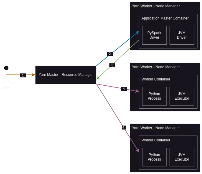
- we submit the job to spark
- spark will then with the help of yarn’s resource manager create the application master in one of the worker nodes. recall how containers are used hadoop 2.x onwards, so this application master would be created inside a yarn / hadoop container
- now, the spark driver will run inside this application master container - remember that since hadoop 2.x, even the application master container is actually just a container running on a worker node, so the driver is also running on a worker node where the node manager is, not the master node where resource manager is
- then, the spark driver will talk to yarn’s resource manager and create more worker containers
- then, spark will spawn executors inside these worker containers
- now, each executor will be responsible for some partition(s) of data, which it loads in its memory as discussed earlier
- while doing all this, spark will take care of rack awareness i.e. assigning executors the partitions in such a way that there is minimum network transfer between hdfs and executor / container
- note for pyspark -
- the driver will have a python component running alongside it. so, if for e.g. using yarn, inside the application master container, there will be a python process and the actual jvm driver. communication between the python process and jvm driver happens using py4j
- if we use functionality / libraries of python not available in pyspark, then the executors too will have a python component running alongside them. so, if for e.g. using yarn, inside the container, there will be a python process and the actual jvm executor
Spark CPU and Memory
- important options which we can include when we submit a job to spark -
- executor-memory, driver-memory - ram
- executor-cores, driver-cores - cpu cores
- num-executors - number of executors
- important - a task uses one slot
- the number of slots in an executor is controlled using the
executor-coresargument, while the number of executors usingnum-executors - remember - an executor is essentially a single jvm process - so, when we say an executor gets 4 cores / 4 slots, it basically means 4 jvm threads for that single executor jvm process
- so, number of tasks that can run in a cluster for a spark job = (number of slots in an executor) * (number of executors)
- note - each slot is essentially a “virtual core” - recall that nowadays, each core can itself be split into virtual cores as well due to hyperthreading
- now, assume that spark computes that it needs 30 tasks but we only have 20 slots in our cluster
- spark is intelligent enough to schedule the 20 tasks and queue the remaining 10 tasks
- till now, we talked about cpu, and now we talk about memory
- when setting memory limits, we have two variations for both executor and driver -
spark.driver.memory,spark.driver.memoryOverhead- my assumption -spark.driver.memoryis same as passing--driver-memoryto spark-submitspark.executor.memory,spark.executor.memoryOverhead- my assumption -spark.executor.memoryis same as passing--executor-memoryto spark-submit
- the memory variant is for the actual jvm driver / jvm executor, while the memory overhead variant is for non jvm processes (like the one needed when using pyspark)
- so, e.g. we set
spark.executor.memoryto 1gb andspark.executor.memoryOverheadto 0.1. spark driver would ask yarn for containers having memory 1.1gb. out of the 1.1gb for a container, 1gb would be allocated for executor jvm process, while the remaining 100mb would be allocated for non jvm processes, like the sidecar needed for pyspark, exchange buffer (refer the read and write buffers here), etc- note - remember the two common cases of memory overhead - exchange and pyspark
- note - this value should of course be lesser than a worker node’s physical memory, otherwise we will get exceptions
Executor Memory Deep Dive
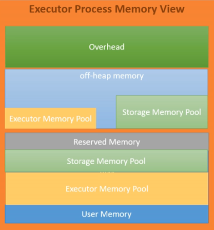
- we can ask for memory using
spark.executor.memory. this is the jvm memory - 300 mb is reserved memory
- remaining memory is divided into spark memory and user memory using
spark.memory.fraction. the default is 0.6 - reserved memory - fixed, used by spark engine
- user memory - used by udfs, some internal metadata, data structures defined by us, and rdds if we use rdd operations directly (not rdds generated internally when we use dataframes)
- spark memory - division is controlled using
spark.memory.storageFraction, which is 0.5 by default- storage memory - caching dataframes. long lived, until we use for e.g.
uncache - executor memory - performing dataframe operations. short lived, as it is freed once the operation is over
- storage memory - caching dataframes. long lived, until we use for e.g.
- the boundary is flexible as well
- storage memory can borrow memory from the executor memory if it has shortage
- e.g. assume storage memory borrows from executor memory
- tasks in executor memory now need some of it back
- now, the cached part in executor memory will be evicted
- this is where setting the
spark.memory.storageFractionis useful
- division of executor memory between tasks -
- e.g.
spark.executor.cores= 4 i.e. we have 4 slots / 4 cores / 4 jvm threads - the executor memory will get divided accordingly as well
- spark is smart enough to do this dynamically - e.g. even if we have 4 cores but two active tasks, and one of them needs more executor memory - spark can divide this executor memory into a ratio of 70-30
- e.g.
- so, for e.g. if our
spark.executor.memoryis 8gb- spark memory is (8000-300) x 0.6 = 4620mb - both storage and executor memory are 2310mb
- user memory is (8000-300) x 0.4 = 3080mb
- finally, an optimization - due to jvm heap memory being not so efficient due to garbage collection etc - spark introduced the concept of offheap memory - so, executor memory / storage memory can use this as well
Job Scheduling
- it governs how different jobs contend with each other for resources. there are two sides to this -
- job scheduling across different applications - dynamic resource allocation
- job scheduling inside the same application - spark schedulers
- just covering from theoretical perspective, how to configure this can be found here
Dynamic Resource Allocation
- e.g. we have a spark job that uses up all the resources in our cluster
- now, we submit another small job
- but, this job cannot run since all the resources have already been used up
- a small job has to wait for the large job to complete
- so, spark has two strategies - static allocation and dynamic allocation
- static allocation - the default. the driver will ask for all the resources for its executors upfront. it will hold on to them for the entire duration till the entire job is over
- when we asked for some executors via the
num-executorsoption, it meant that the spark driver would hold on to these resources for the entire duration of the job - however, the number of executors the stages actually use can change dynamically
- remember - number of executors used in a stage depends on the number of tasks a stage has
- so, we can instead use dynamic resource allocation - where instead of us manually specifying the number of executors to use, it is determined dynamically for every stage
- by default, static allocation is used, but we should consider using dynamic allocation if we are using a shared cluster for multiple jobs
Spark Schedulers
- if our spark application has multiple jobs -
df1.join(df2).count() df3.join(df4).count() - by default, spark driver would execute this code synchronously. so, first all jobs for the first line would finish and then the all jobs for the second line would start and finish
- however, what if we use multithreading? - e.g. something like this -
Thread t1 = new Thread(() -> df1.join(df2).count()); Thread t2 = new Thread(() -> df3.join(df4).count()); t1.start(); t2.start(); t1.join(); t2.join(); - this means that the jobs for both would be triggered in parallel
- this is what we might actually want as well - what is the point of stalling the second job for the first job?
- however, when kicking off the jobs in parallel like this, they will contend with each other for resources
- solution - by default, spark uses the fifo scheduler, but we can ask it to use the fair scheduler as well
- fifo scheduler - the first job gets priority. it gets all the resources for itself. then the second job gets the leftover, and would be stalled if not enough resources are available
- fair scheduler - assign resources to tasks in a round robin fashion. all issues like starvation (short job waiting for a long running job) etc are prevented
Transformations and Actions
- spark dataframes are immutable i.e. the transformations we perform when using the api results in new dataframes, and the old one stays as is
- we tell spark driver the transformations we would like to do
- these transformations are simple sql statements - e.g. filter where age > 40, projection of columns, grouping, etc
- each transformation then results in a new dataframe
- transformations can be further categorized into narrow transformation and wide transformation
- narrow transformation - each partition of data can be processed independently. a transformation on one partition is independent of a transformation on another partition. e.g. filtering
- wide transformation - partitions need to be repartitioned. e.g. in group by, all rows belonging to the same group need to be brought into the same partition. this process of repartitioning of data for a wide transformation is called a shuffle
- execution plan - we write the transformations one by one using a builder pattern. but spark might not execute the operations in the same way - it will construct an execution plan, which is an optimized version of our transformations - e.g. if we filter then use project, it would move the projection before the filtering
- lazy evaluation - spark will not execute the transformations immediately - it will build the execution plan described above and wait for us to call an action. actions include
read,write,collect,show. the moment we call an action, the execution plan is triggered, and we see a job collectwill basically collect all the data in the driver. so, be mindful of out of memory exceptions when performing this operation
Jobs, Stages and Tasks
- our entire spark application is broken down into jobs
- a job is triggered only once an action is encountered (recall lazy evaluation)
- jobs are further broken down into stages
- stages are further broken down into tasks
- so, tasks are the unit of work
- a task basically executes on one slot of executor and is responsible for a partition of data
- a task is basically a bunch of narrow transformations - so, all task of a stage can operate on its partition of data independently
- therefore, all the tasks of a single stage operate in parallel
- each wide transformation results in a new stage, due to the repartitioning that is needed
- before the tasks of a next stage start, all tasks of the previous stage should complete, because that was the entire point behind wide transformation - it depends on all the previous stage’s partitions and not just one
- when going from one stage to another, since data is being shuffled / repartitioned, data is temporarily written to a buffer which spark calls exchange (recall the use of memory overhead)
- so, the idea probably is to wait for all tasks of a stage to complete and then with the help of exchange, get the right partition of data to the right executor and finally kick off the tasks of the new stage
- this process of copying data from the write exchange to the read exchange is called shuffle / sort

- spark creates 3 jobs for the below snippet -
- one job to read the data
- one job for inferring the schema etc
- one last job for collect
- so, the number of jobs was equal to the number of actions we have. an internal action for inferring the schema resulted in the extra job
- the number of partitions created after a wide transformation etc is controlled by
spark.sql.shuffle.partitions - however, we can midway our transformations, repartition the dataframe using
repartition - so, both operations below, repartition and group by cause the shuffle sort
- this means we will have 3 total stages for the third job
bestsellers = (
  spark.read
  .format('csv')
  .option('header', 'true')
  .option('inferSchema', 'true')
  .load('data/bestsellers.csv')
)

counts_by_genre = (
  bestsellers.repartition(2)
  .where(col('User Rating').__gt__(4.5))
  .groupBy('Genre')
  .count()
)

print(counts_by_genre.collect())
- spark 3.x has changed - aqe is enabled by default in spark 3.x and above
- this means each stage results in a new job
- so, while spark 2.x should have had 3 stages for third job, we now have 3 jobs for it instead, resulting in a total of 5 jobs now
- skipped stages -
- 4th job has one skipped stage, since 3rd job executed it already
- 5th job has two skipped stages, since 3rd and 4th jobs executed it already
Writing Tests
- for getting started, just break down everything into functions
def read_bestsellers(spark, path) -> DataFrame: return ( spark.read .format('csv') .option('header', 'true') .option('inferSchema', 'true') .load(path) ) - now, we can simply use unittest
class BestSellersTransformationsTest(unittest.TestCase): def setUp(self): self.spark = ( SparkSession.builder .appName('spark') .master('local[*]') .getOrCreate() ) def test_read(self): bestsellers = read_bestsellers(self.spark, 'data/bestsellers_mock.csv') self.assertEquals(len(bestsellers.collect()), 9) - important - notice the use of collect - technically, this helps collect everything in the driver, which is not a problem since tests run against small, mocked pieces of data
Debugging and Configuring Spark
- debugging spark is not easy - all the code we write is first converted into an execution plan and is lazily evaluated
- so, when we place debug pointers in our code, we are just stepping through the driver thread (which is not even doing anything). we are not stepping through the executor thread actually performing those transformations
- we can however use lambda accepting transformations like
map,flatMap,forEach, etc - when we place debug pointer inside these lambdas, we will be able to see the executor thread performing them
- logs are the best way of debugging a production spark application, which is running in a distributed environment
- we use log4j2 for to provide the appropriate log configuration, since that is used by hadoop / spark
- we can specify the log4j2.properties file to use. this can be cluster wide or application specific, depends on use case
- now, we can configure our file and console appenders. e.g. -
- we set root level to send warn level (so warn and error logs) to console appender
- we set application level to send info info level logs to both console and file appender
log4j.rootCategory=WARN, console log4j.logger.learning.spark.examples=INFO, console, file - while using the file appenders, we need to ensure that the path is inside
spark.yarn.app.container.log.dir. this is because our logs are distributed across machines (executors and drivers), and doing this ensure yarn collects our logs from the different machines for uslog4j.appender.file.File=${spark.yarn.app.container.log.dir}/${logfile.name}.log - we can use log4j inside pyspark as follows -
log4j = spark._jvm.org.apache.log4j logger = log4j.LogManager.getLogger('learning.spark.examples') logger.info('hello world') logger.error('hello world') logger.warn('hello world') - finally, the starter file i believe we can use to configure spark is here. we can configure pyspark to use this file as follows -
conf = SparkConf() conf.set('spark.driver.extraJavaOptions', '-Dlog4j.configuration=file:log4j2.properties') spark = ( SparkSession.builder .config(conf=conf) # ... ) - note - we had to do this because we are using the local cluster manager / or if we want application specific configuration. we could also have configured this in the spark conf directory directly, and then it would have applied to all jobs submitted to the spark cluster
- spark can be configured from the following four places -
- environment variables
- spark home \ conf \ spark-defaults.conf
- spark-submit command line options
- spark conf object
- note that this is also the order of increasing precedence i.e. anything we set via the spark-submit command line takes precedence over the same thing specified via environment variables
- the first two methods apply cluster wide, while the second two are application specific
Spark Structured APIs
- rdd stands for resilient distributed dataset
- resilient because if for e.g. there is a failure in one of the executors, spark knows how to load the partitions the failed executor was responsible for into a new executor
- distributed because spark partitions the data into smaller chunks and processes them in parallel
- spark structured apis comprises of
- sql
- dataframe
- dataset
- using structured apis vs rdd -
- structured apis basically use rdd underneath
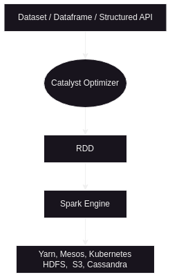
- spark asks us to use structured apis where possible, since there is a catalyst optimizer (also called tungsten) sitting in between structured apis and rdd, so we lose out on the optimizations when using rdd directly
- use rdd only for specific use cases like custom partitioning
- apis are also different - rdd apis do not have out of the box support for different file formats like csv, json, etc like dataframe reader
- using a dataframe vs a dataset -
- dataset will have compile time safety - using
.filter((person) -> person.age > 40)has compile time safety unlike.where(col("age").gt(40)) - dataset is less optimal when compared to dataframe - serialization is an important step in distributed computing. dataset serialization will use java serializers, while dataframe serialization will be able to use tungsten underneath, which is more performant
- i believe datasets are not even available in pyspark, since it is a non jvm language
- in jvm languages, for e.g. java, dataframe is actually
Dataset<Row>, while dataset would actually meanDataset<Pojo>
- dataset will have compile time safety - using
- finally, we can also use sql, which would just be a string. sql i believe works just like dataframe, so there should be no performance impact there. however, we loose out on programming specific features like logging, compile time safety, unit testing, etc
- based on everything above, i will probably use dataframe all the way. i would also use the apis and not sql, since it has a bit better compile time safety / auto complete as compared to writing sql strings
- spark engine - this sits on top of the chosen cluster manager and storage. recall how spark has flexibility for both
- first we typically create the spark session when running locally. it is already available to us by default when using databricks. the alternative to the builder pattern is creating the spark config object manually -
conf = SparkConf() conf.set('spark.master', 'local[*]') conf.set('spark.app.name', 'basics') spark = ( SparkSession.builder .config(conf=conf) .getOrCreate() ) - note - remember the lines to create the basic spark session / read a file. it is asked in interviews
Execution Plan / Catalyst Optimizer Working
- the catalyst optimizer works internally in following steps
- or we can say that spark executes the execution plan in the following steps
- generate an ast or abstract syntax tree. any errors in our field names, data types, sql function usage, etc would be caught here
- now we will have a logical plan
- perform optimization on our logical plan. the optimization here includes techniques like -
- predicate pushdown - push filtering operations earlier to reduce the amount of data transfer
- partition pruning - when writing to internal sources, we can specify partitioning scheme, and then there will be a different directory for each partition. this has been discussed in data sources. predicate pushdown can go up to as early as only reading some partitions of data when loading the data into dataframes
- projection pruning - push projection operations earlier to reduce the amount of data transfer
- generate a bunch of physical plans, and associate a cost with each of them. e.g. one plan uses shuffle join, another uses broadcast join
- finally, a cost model evaluates the most optimal physical plan
- wholestage code generation - generate the bytecode to run on each executor
- note - i think wherever dag (directed acyclic graph) is mentioned, it refers to this entire process

Data Sources - Reading
- data sources in spark can be external or internal
- external - external to spark. some notable ones include
- jdbc data sources - oracle, ms sql, postgres, mysql
- no sql - cassandra, mongo db
- cloud data warehouses - snowflake, redshift
- streaming sources - kinesis, kafka
- internal - this can be either hdfs or cloud based storage e.g. s3 (preferred). from a code perspective, nothing changes much here
- for internal source, there are several file formats which we have to consider. again, spark supports various file formats like parquet, json, csv, avro, etc
- we can also write using spark tables apart from the file formats mentioned above. recall that it would store store the metadata in the storage as well using the metastore
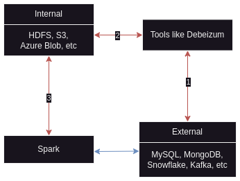
- there are two ways to access external sources -
- ingest using external tools to write data from external sources to internal sources. data goes unmodified from different sources into internal sources. then spark reads from these internal sources directly
- make spark directly read from these different external sources
- batch processing prefers first option because for e.g. our db capacity was provisioned with oltp workloads in mind, and might not be optimized for spark based big data workloads. thus, it helps decouple the two from performance, security, etc perspective
- stream processing prefers second option
![spark architecture]()
- the different tools to my knowledge include kafka by itself (probably the most common), talend, debezium, informatica
- the dataframe reader makes it so that interacting with all kinds of sources / formats feels the same
- schema -
- for file formats like csv, either it can be defined explicitly using
schema(preferred), or it can infer the schema automatically (prone to errors) - for file formats like avro / parquet, the schema is a part of the file itself and therefore we do not need to specify the schema explicitly. so best case would be to try and use parquet / avro formats where possible. parquet is the default in spark
- for file formats like csv, either it can be defined explicitly using
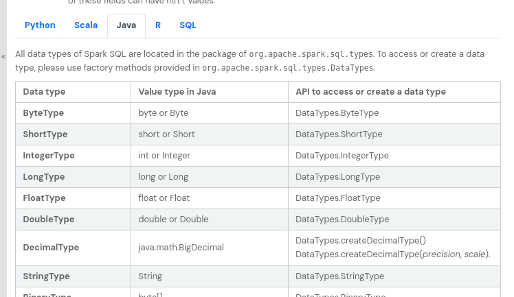
- spark has its own data types, and they map to different types specific to the language we use, e.g. we can see how spark types map to java types here
![spark to java types]()
- we access the dataframe reader using
spark.read - we specify the type using
format - we provide configuration using
option - we can print the schema by chaining
printSchema() - if we do not even use
inferSchema, all types are a string. so, we useinferSchema-flights = ( spark.read .format('csv') .option('header', 'true') .option('inferSchema', 'true') .load('data/flight-time/flight-time.csv') ) flights.printSchema() # |-- FL_DATE: string (nullable = true) # |-- OP_CARRIER: string (nullable = true) # |-- ORIGIN: string (nullable = true) # |-- DEST: string (nullable = true) # |-- CANCELLED: integer (nullable = true) # |-- DISTANCE: integer (nullable = true) - issue - while distance etc were parsed correctly as an integer, the
FL_DATEfield is parsed as a string - so, we set the schema explicitly
- we can also provide a mode, which determines the behavior when spark encounters a malformed record. it can be -
- permissive (default) - make all columns null and place the record in a new column
_corrupt_record - drop malformed - ignore the malformed records
- fail fast - terminate the program
- permissive (default) - make all columns null and place the record in a new column
- note - now that we specify the schema explicitly, we might also want to get an error if this schema is not satisfied. so, we set the mode to fail fast this time around as well
- finally, also note how we specified the date format in configuration itself, otherwise spark will give an error. for column specific configuration (e.g. if two different columns have differently formatted dates), maybe we can use
to_dateto convert from string to date type during transformationsschema = StructType([ StructField("FL_DATE", DateType()), StructField("OP_CARRIER", StringType()), StructField("ORIGIN", StringType()), StructField("DEST", StringType()), StructField("CANCELLED", IntegerType()), StructField("DISTANCE", IntegerType()) ]) flights = ( spark.read .format('csv') .option('header', 'true') .option('mode', 'FAILFAST') .option('dateFormat', 'M/d/y') .schema(schema) .load('data/flight-time/flight-time.csv') )
Data Sources - Writing
- sinks work in the same way as sources in spark - they can be internal or external, preference should be based on type of processing - batch or stream
- the default format used by spark is parquet if not specified
- the mode can be -
- append - append to the existing data
- overwrite
- error if exists
- ignore - write if location is empty, ignore otherwise
- for using avro, we have to add the spark avro dependency separately, which i added as follows. spark automatically takes care of downloading the package etc
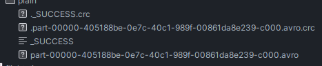
conf = SparkConf() conf.set('spark.jars.packages', 'org.apache.spark:spark-avro_2.12:3.5.1') spark = ( SparkSession.builder .appName('writing') .master('local[*]') .config(conf=conf) .getOrCreate() ) - so, i see the following files when i use the code below -
flights.write \ .format('avro') \ .mode('overwrite') \ .save('data/flight-time/out/plain')![simple output]()
- note -
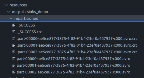
df.writereturns the dataframe writer - by default, all our partitions are written to separate files. e.g. if we have 3 partitions / executors, we will get 3 different files for the data. recall that we can also repartition our data using repartition
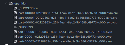
flights \ .repartition(3) \ .write \ .format('avro') \ .mode('overwrite') \ .save('data/flight-time/out/repartition')![repartitioned output]()
- however, partitioning blindly might not be always suitable for our use case - while this gives us ability for parallel processing in future, we loose out on benefits like partition elimination
- so, my understanding - partition by is when we want to write the output and make it optimized for future jobs that might read this output. however, repartition can help with optimizing the current job itself
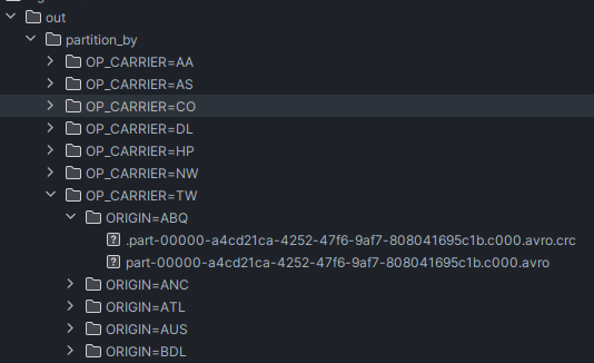
- note how directories for origin are nested inside directories for carrier
flights.write \ .format('avro') \ .mode('overwrite') \ .partitionBy('OP_CARRIER', 'ORIGIN') \ .save('data/flight-time/out/partition_by')![partition by output]()
- also, remember that partition by and the methods like bucket by we see in future are applicable while writing, which is why we chain it to the dataframe writer, but repartition is chained to the dataframe itself
- we can also chain
maxRecordsPerFile. it is useful when there are some partitions that become too big for spark to process. e.g. in the above example, if for carrier nw and origin den, the number of flights were too many, by using this option, this directory too will contain multiple files - why use bucketing - since partitioning results in a unique directory for each value, partitioning by a column having too many unique values might not be a good idea, since it would result in too many directories (partitions) with too less data. so, we can instead use bucketing for columns having too many unique values
- how it works - we specify the number of buckets and the column to bucket using. then, spark will do hash(column_value) % number_of_buckets to get the bucket in which the row should be stored
- sorting - sorting can further improve the performance - e.g. if we had to perform joins, and the data is already sorted on the columns used for join, we can skip the sort phase in the shuffle join (described later)
flights.write \ .bucketBy(2, 'OP_CARRIER', 'ORIGIN') \ .sortBy('OP_CARRIER', 'ORIGIN') \ .mode('overwrite') \ .save('data/flight-time/out/bucket_and_sort_by') - however, i got the following exception on running the above -
'save' does not support bucketBy and sortBy right now
Spark + Hive
- so, we have to use
saveAsTable. my understanding - till now, we were simply storing data as normal files, and they were accessible like a regular directory structure, but for bucketing and sorting, we need to bring in “database support” of spark. we discussed this difference here - since spark too has concepts of database and tables, there are two things spark needs to store -
- the actual data - this is what we have seen till now, when for e.g. we saw files being stored inside folders (i.e. partitions)
- the metadata - the table name, database name, etc. this is stored in something called metastore. spark borrowed this from hive
- there are two kinds of tables in spark -
- managed tables - spark will manage both the metadata and the actual data. by default, the actual data is stored inside
spark.sql.warehouse.dir. when we for e.g. drop a table, both the metadata and the actual data get deleted - unmanaged tables - also called external tables. spark will only manage the metadata. when creating a table, we specify the location of the actual data. useful when for e.g. the actual data already exists somewhere and is not managed by us. when we for e.g. drop a table, only the metadata is deleted, and the actual data is untouched
- managed tables - spark will manage both the metadata and the actual data. by default, the actual data is stored inside
- managed tables are preferred - we can do optimizations like bucketing and sorting. with unmanaged tables, we have to rely on the existing data structure. we need unmanaged tables when we need to perform spark operations on already existing data
- my thought - one technique might be to use spark itself to read from unmanaged tables but write data to managed tables at the back of it?
- we need to enable the support for hive as follows when creating the spark session
spark = ( SparkSession.builder .appName('pyspark') .master('local[*]') .enableHiveSupport() .getOrCreate() ) - then, we need to create the database we want to save to incase it does not already exist -
spark.sql('create database if not exists airline_db') print(spark.catalog.listDatabases()) # [Database(name='airline_db', # catalog='spark_catalog', description='', # locationUri='file:/home/shameek/Desktop/library/pyspark-batch-processing/spark-warehouse/airline_db.db') # Database(name='default', # catalog='spark_catalog', description='Default Hive database', # locationUri='file:/home/shameek/Desktop/library/pyspark-batch-processing/spark-warehouse')] - i see the following directories for metastore and warehouse created automatically -
![]()
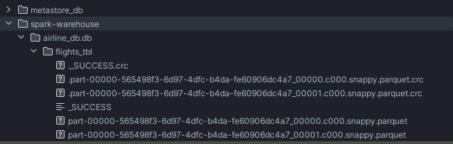
- finally, we write a dataframe as follows. note - notice how we do not provide the path parameter, since it is managed table territory, therefore the
spark.sql.warehouse.dirwill be used, and we callsaveAsTable(db_name.table_name)instead ofsave()flights.write \ .mode('overwrite') \ .bucketBy(2, 'OP_CARRIER', 'ORIGIN') \ .sortBy('OP_CARRIER', 'ORIGIN') \ .saveAsTable('airline_db.flights_tbl') print(spark.catalog.listTables('airline_db')) # [Table(name='flights_tbl', # catalog='spark_catalog', namespace=['airline_db'], description=None, # tableType='MANAGED', isTemporary=False)] - notice the two files for storing the data, since we specified the number of buckets to be 2
![partition by output]()

Transformations
- for transformations, we have two options -
- column object expressions - python
- sql - strings
- i prefer column object expressions since we get autocomplete help from the ide, can maintain formatting of code, etc
- for specifying columns in transformations, either use column_name directly as a string, or use
col('column_name') - note - we cannot use both methods in the same transformation
- use
selectto select a subset of columns,dropto drop a subset of columns - a function for adding a unique identifier to each record -
monotonically_increasing_id. this number would be unique across all partitions but remember that it would not necessarily be continuous - usual sql constructs like renaming using
alias, changing data type usingcast, etc are available explode- e.g. our record contains an array field. this field will ensure our result contains a record for each element of the array. e.g. if our input has 2 elements in the array for the first record, and 3 elements in the array for the second record, the output will have 5 recordswithColumn- modify an existing column / create a new column name using the specified expressioncalls = ( calls .withColumn('Call Date', to_date('Call Date', 'M/d/y')) .withColumn('Call Date Year', year('Call Date')) .withColumn('Call Date Week', weekofyear('Call Date')) )withColumnRenamedto rename columns - e.g. during joining, both order line and product can have a quantity - one can denote the quantity ordered, while the other can denote the quantity in stock
Example 1
input - assume dobDf dataframe has the following rows
day month year 28 1 2002 23 5 81 12 12 6 7 8 63 23 5 81 - transformation -
dobDf = (
  dobDf
  .withColumn(
    'normalized_year',
    when(col('year') <= 24, col('year') + 2000)
    .when(col('year') <= 99, col('year') + 1900)
    .otherwise(col('year'))
  )
  .withColumn('dob', concat_ws('/', 'day', 'month', 'normalized_year'))
  .withColumn('dob', to_date('dob', 'd/M/yyyy'))
)
output -
day month year normalized_year dob 28 1 2002 2002 2002-01-28 23 5 81 1981 1981-05-23 12 12 6 2006 2006-12-12 7 8 63 1963 1963-08-07 23 5 81 1981 1981-05-23
Example 2
- assume we have a log file that looks like this -
83.149.9.216 - - [17/May/2015:10:05:03 +0000] "GET /presentations/logstash-monitorama-2013/images/kibana-search.png HTTP/1.1" 200 203023 "http://semicomplete.com/presentations/logstash-monitorama-2013/" "Mozilla/5.0 (Macintosh; Intel Mac OS X 10_9_1) AppleWebKit/537.36 (KHTML, like Gecko) Chrome/32.0.1700.77 Safari/537.36" 83.149.9.216 - - [17/May/2015:10:05:43 +0000] "GET /presentations/logstash-monitorama-2013/images/kibana-dashboard3.png HTTP/1.1" 200 171717 "http://semicomplete.com/presentations/logstash-monitorama-2013/" "Mozilla/5.0 (Macintosh; Intel Mac OS X 10_9_1) AppleWebKit/537.36 (KHTML, like Gecko) Chrome/32.0.1700.77 Safari/537.36" 83.149.9.216 - - [17/May/2015:10:05:47 +0000] "GET /presentations/logstash-monitorama-2013/plugin/highlight/highlight.js HTTP/1.1" 200 26185 "http://semicomplete.com/presentations/logstash-monitorama-2013/" "Mozilla/5.0 (Macintosh; Intel Mac OS X 10_9_1) AppleWebKit/537.36 (KHTML, like Gecko) Chrome/32.0.1700.77 Safari/537.36" - when we try reading it in, we use text format, and everything is squashed into one attribute, since python cannot automatically parse it
logs = ( spark.read .format('text') .load('data/apache_logs.txt') ) logs.show() # +--------------------+ # | value| # +--------------------+ # |83.149.9.216 - - ...| # |83.149.9.216 - - ...| # |83.149.9.216 - - ...| - we want to extract its individual fields. we can use the
regexp_extractfunction, which helps us extract the matched specific group - in the output, notice how the referrer column has the entire url, but we wanted to extract the domain only (to for e.g. be able to group using this later). so, we use
substring_index. we specify a delimiter and n, and we get back the substring from the beginning up to and excluding the nth delimiter - finally, a useful debugging tip - notice the use of the truncate = false to avoid truncating the column values when logging the dataframe
log_regexp = r'^(\S+) (\S+) (\S+) \[([\w:/]+\s[+\-]\d{4})\] "(\S+) (\S+) (\S+)" (\d{3}) (\S+) "(\S+)" "([^"]*)'

logs = (
  logs
  .withColumn('ip', regexp_extract('value', log_regexp, 1))
  .withColumn('date', regexp_extract('value', log_regexp, 4))
  .withColumn('request', regexp_extract('value', log_regexp, 6))
  .withColumn('referrer', regexp_extract('value', log_regexp, 10))
  .withColumn('referrer_domain', substring_index('referrer', '/', 3))
  .drop('value')
)

logs.show(truncate=False)

# +------------+--------------------------+----------------------------------------------------------------------------------+---------------------------------------------------------------+-----------------------+
# |ip          |date                      |request                                                                           |referrer                                                       |referrer_domain        |
# +------------+--------------------------+----------------------------------------------------------------------------------+---------------------------------------------------------------+-----------------------+
# |83.149.9.216|17/May/2015:10:05:03 +0000|/presentations/logstash-monitorama-2013/images/kibana-search.png                  |http://semicomplete.com/presentations/logstash-monitorama-2013/|http://semicomplete.com|
# |83.149.9.216|17/May/2015:10:05:43 +0000|/presentations/logstash-monitorama-2013/images/kibana-dashboard3.png              |http://semicomplete.com/presentations/logstash-monitorama-2013/|http://semicomplete.com|
# |83.149.9.216|17/May/2015:10:05:47 +0000|/presentations/logstash-monitorama-2013/plugin/highlight/highlight.js             |http://semicomplete.com/presentations/logstash-monitorama-2013/|http://semicomplete.com|
User Defined Functions
- we can register custom functions to use inside spark
- e.g. assume we have a survey df. the gender column in there does not have a standardized value
survey.select('gender').distinct().show() # non-binary, Make, F, Genderqueer, Man, Male (CIS), m, Female, Agender, Mal, f, maile, Trans-female, Nah, Cis Female, woman, Female, Cis Man, female, M - assume we want to standardize it to male, female or unknown. we can create a custom function for this -
def parse_gender(gender): female_regexp = r'^f$|fem|wom' male_regexp = r'^m$|mal|man' if re.search(female_regexp, gender.lower()): return 'Female' elif re.search(male_regexp, gender.lower()): return 'Male' else: return 'Unknown' - now, we can use this custom function in our transformations as follows -
parse_gender_udf = udf(parse_gender, StringType()) survey = ( survey .withColumn('parsed_gender', parse_gender_udf('gender')) ) survey.select('gender', 'parsed_gender').distinct().show() # +--------------------+-------------+ # | gender|parsed_gender| # +--------------------+-------------+ # | Androgyne| Unknown| # | Agender| Unknown| # | Male (CIS)| Male| # | Woman| Female| # | Male | Male| # | F| Female| # | Female| Female| # | M| Male| # .... - the udf function receives the custom function and return type, and returns the registered udf
- our function is serialized and sent over to all the executors
- however, we still cannot use it if we were using sql strings instead of column object expressions
- to be able to use it inside sql, we need to instead register it to the sql function catalog using the following method -
spark.udf.register('parse_gender_udf', parse_gender, StringType())
Aggregations
- simple aggregations - gives a one line summary for the complete dataframe
stats = invoices.select( count('*').alias('total count'), count('Description').alias('total non null descriptions'), avg('UnitPrice').alias('average unit price'), count_distinct('InvoiceNo').alias('distinct invoices') ) # +-----------+---------------------------+------------------+-----------------+ # |total count|total non null descriptions|average unit price|distinct invoices| # +-----------+---------------------------+------------------+-----------------+ # | 541909| 540455| 4.611113626088501| 25900| # +-----------+---------------------------+------------------+-----------------+ - note - difference between
count(*)vscount(column_name)-count(column_name)gives us the total number of non null values for the column, whilecount(*)gives us the total number of rows - grouping aggregations - we can also perform groupings using
groupBystats_by_invoice = ( invoices .groupBy('InvoiceNo') .agg( sum(col('Quantity')).alias('total quantity'), round(sum(col('Quantity') * col('UnitPrice')), 2).alias('invoice value') ) ) stats_by_invoice.show() # +---------+--------------+-------------+ # |InvoiceNo|total quantity|invoice value| # +---------+--------------+-------------+ # | 536596| 9.0| 38.09| # | 536938| 464.0| 1680.88| # | 537252| 31.0| 26.35| # | 537691| 163.0| 310.57| # | 538041| 30.0| 0.0| - note - when we chained
groupBy, it returns a grouped data object, and when we again chainedaggto it, it was converted back to our usual dataframe - tip - we can extract complex column object expressions to variables to improve readability -
invoice_value = round(sum(col('Quantity') * col('UnitPrice')), 2).alias('InvoiceValue') # ... .agg( invoice_value, # ... ) - window aggregations - e.g. we need the running total by week for every country. three things to keep in mind for windowing aggregations -
- identify the partitioning columns - e.g. here, restart the running total for every country
- identify the ordering of columns - e.g. here, ensure that the data is ordered by the week number, week 3’s running total = week 1’s sale + week 2’s sale + week 3’s sale, and this is only possible when we order by week
- identify the window bounds - e.g. here, it starts at the first record and ends at the current record, like described in the week 3 example above. options for window bounds include
unboundedFollowing,unboundedPreceding,currentRow, etc. we will need unbounded preceding and current. we can also specify integers here i believe - (-2) for the two rows before etc
- output would be automatically sorted by week number based on the window we specified, and it would have the running total column added to it, which automatically resets for every country
- important note i keep forgetting - window functions basically add a column to the current table. they do not somehow reduce the number of rows like traditional group bys. this thought might be important when coming up with solutions
# input dataframe snippet
# +---------------+----------+-----------+-------------+------------+
# |        Country|WeekNumber|NumInvoices|TotalQuantity|InvoiceValue|
# +---------------+----------+-----------+-------------+------------+
# |           EIRE|        17|          1|          163|       362.9|
# |Channel Islands|        46|          1|           78|      211.63|
# |         France|        10|          1|          325|      712.85|
# |         France|         6|          1|          301|      455.02|
# |        Germany|        17|          2|          452|     1172.55|

window_spec = (
  Window
  .partitionBy('Country')
  .orderBy('WeekNumber')
  .rowsBetween(Window.unboundedPreceding, Window.currentRow)
)

stats_by_country_and_week = (
  stats_by_country_and_week
  .withColumn('RunningInvoiceTotal', sum('InvoiceValue').over(window_spec))
)

stats_by_country_and_week.show()

# output dataframe snippet
# +---------+----------+-----------+-------------+------------+-------------------+
# |  Country|WeekNumber|NumInvoices|TotalQuantity|InvoiceValue|RunningInvoiceTotal|
# +---------+----------+-----------+-------------+------------+-------------------+
# |Australia|      NULL|         26|        33035|    46476.38|           46476.38|
# |Australia|         1|          2|         4802|     7154.38|           53630.76|
# |Australia|         2|          3|          394|       721.1|           54351.86|
# |Australia|         3|          3|          338|      757.55|           55109.41|
# |Australia|         7|          1|         8384|    14022.92|           69132.33|
Joins
- bringing “left” and “right” dataframe together
- we combine them using the join expression and the join type
order_details = orders.join( products, products.prod_id == orders.prod_id, 'inner' ) - order schema - (order_id, prod_id, unit_price, qty)
- product schema - (prod_id, prod_name, list_price, qty)
- therefore, the joined table’s schema - (order_id, prod_id, unit_price, qty, prod_id, prod_name, list_price, qty)
- note how the joined table’s schema contains two columns for quantity
- one is from the product - it indicates number of units in stock
- one is from the order - it indicates quantity of product ordered
- assume we wanted to select only some columns (only order’s quantity, not product’s quantity) -
order_details = ( orders.join( products, products.prod_id == orders.prod_id, 'inner' ) .select('order_id', 'prod_name', 'unit_price', 'qty') ) - we get the following exception -
[AMBIGUOUS_REFERENCE] Reference 'qty' is ambiguous, could be: ['qty', 'qty']. - how it works - we pass column names, internally spark converts to it the right internal identifier. when we pass qty, it probably finds two identifiers and hence gets confused
- some solutions -
- rename columns before joining (
withColumnRenamed)products = products.withColumnRenamed('qty', 'product_qty') - drop one of the ambiguous columns - after or before the join, doing after the join here
.join(...) .drop(products.qty) .select('order_id', 'prod_name', 'unit_price', 'qty') - similar to above - specify explicitly which dataframe’s quantity to use - notice the end of the select clause
.join(...)
.select('order_id', 'prod_name', 'unit_price', products.qty)
- rename columns before joining (
- when we use an outer join like left, we might receive nulls for some columns. to get rid of the nulls, we can use coalesce, which will set the final value to the first non null value from the list it receives. e.g. below, we do a left join to get all the orders. prod_name comes from the product dataframe. if the product for an order is missing, prod_name would be null. so, we tell spark to use prod_id of order dataset if prod_name of the product dataset is missing
order_details = ( orders.join( products, products.prod_id == orders.prod_id, 'left' ) .withColumn('prod_name', coalesce('prod_name', orders.prod_id)) .select('order_id', 'prod_name', 'unit_price', products.qty) ) - tip for clean code - note how we write each of the chaining all in one place. we can for e.g. extract join conditions etc to variables, just like we saw for column object expressions in transformations
- there are two kinds of joining techniques used by spark - shuffle join and broadcast join
Shuffle Joins
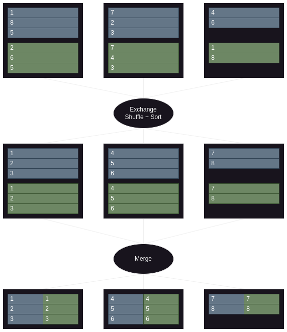
- imagine when we have two datasets with 3 partitions, and we have three executors
- so first a shuffle + sort happens to ensure that the same keys from both datasets belong to the same executor
- now, we perform a sort merge join to join the two datasets
- refer diagram here to recall breakdown of exchange and shuffle + sort
- small note - i am defaulting to thinking of shuffle joins as shuffle sort merge joins. there is another variation - shuffle hash joins, which is less optimal when compared to shuffle sort merge joins, so i am ignoring shuffle hash joins for now
Optimizing Shuffle Joins
- reduce data being joined - because this shuffle and sort process is of course the bottleneck and can cause out of memory like issues, we should consider techniques like filtering (basically reducing) the amount of data we are joining, performing aggregations before joining, etc. basically, code intelligently
- maximize parallelism - the maximum parallelism possible when performing a join is the minimum of the three parameters below, so try maximizing the three parameters below -
- maximum number of executors our cluster allows. recall it can be controlled via
--num-executors spark.sql.shuffle.partitions- this determines the number of partitions after a shuffle i.e. after a wide transformation happens. the default value of this is 200. so, in case of join, this will give the number of partitions of the joined dataset?- number of unique keys in the datasets involved in the join - we need to handle key skews / hot partitions. e.g. we try joining orders with products. we realize that some products sell a lot, while others not so much. this means some products can cause out of memory errors, and we need to use some optimizations here. i think one of the solutions here is salting
- maximum number of executors our cluster allows. recall it can be controlled via
Broadcast Joins
- shuffle joins are used when we join two large datasets
- however, we can use broadcast joins when either (or maybe both) the datasets are small
- assume the smaller dataset can be stored inside one partition, while the larger dataset has 200 partitions
- if using the shuffle join technique, first all of the 200 + 1 partitions will be sent for shuffle and sort
- this means there is network transfer involved to first send the data to exchanges and then load it back in a sorted manner into the executors
- however, in the broadcast join technique, the partitions of the larger dataset can stay where they were, and the smaller dataset can be copied over to all the executors having the larger dataset partitions
- this way, we avoid having to move (shuffle) the larger dataset’s partition over the network
- essentially, we are broadcasting the smaller dataset to all the executors having the larger dataset
- important - the driver and executor memory should be > than the size of the smaller dataset, so that it can fit inside the memory
- notice how below the larger dataset stays as it is, and is not even sorted. unlike shuffle join, broadcast join is a hash join always. recall in shuffle joins, we have the concept of both hash joins (rarely used) and sort merge joins
![broadcast join working]()
- the threshold which decides when to use a broadcast join is
spark.sql.autoBroadcastJoinThreshold, which is 10mb by default - we can also provide spark the hint to use broadcast join like so, if we are not happy with the defaults -
flightsDf1.join(broadcast(flightsDf2), ... - note - to confirm all this, go to http://localhost:4040/ -> Sql / Dataframe tab -> select the sql query
- we can tell from this if an exchange was involved or we skipped it by using bucketed joins, if shuffle join was used or broadcast join was used, etc

Bucketed Joins
- if the datasets are already bucketed and sorted using the keys involved in the join, we will not have to rely on the shuffle sort done by spark at all
- the idea is to store the datasets in bucketed fashion before the join starts
- we basically prepone the shuffling activity
- when we load the datasets and perform the join, there would be no shuffling involved
- it would be a plain sort merge join without the shuffle sort - the spark ui would show that no shuffle was involved
- probably bts, spark is smart enough to realize that the dataframes are bucketed the same way, and hence it will colocate them on the same executor from the get go to avoid that shuffle
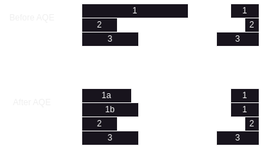
Spark AQE
- aqe - adaptive query execution
- it includes optimizations discussed below
- set
spark.sql.adaptive.enabledto true for this (it should be enabled by default in new versions), and rest of the optimizations discussed in this sections will be automatically enabled - working principle - spark computes statistics during the shuffle operation - things like no. of rows in each unique group if we are doing group by etc
- there are three parts to this aqe -
- crazy granular configurations can be seen here for all three optimizations, use documentation for specific configuration, just learning things from theoretical perspective for now
Dynamically Deciding Shuffle Partitions
- earlier, after a wide transformation, for e.g. group by, the number of output partitions from a stage would be =
spark.sql.shuffle.partitions(default 200), but lets say we set it to 10 - what if i only have e.g. 5 groups after a group by statement?
- spark would still create a total of 10 partitions, therefore 10 tasks in the subsequent stage
- now, our spark job would eat up the resources for 5 empty tasks as well
- remember that for a wide transformation, spark stalls all the tasks of its previous stage, so the empty tasks are just sitting idle
- this optimization by aqe resolves this issue
- spark will look at the number of unique groups, and then dynamically adjust the number of output partitions
- now, assume one of the partitions was relatively larger
- spark used one task for one partition of data
- spark would complete all the tasks except this one quickly
- again, remember that for a wide transformation, spark stalls all the tasks of its previous stage, so the tasks that get over quickly are just sitting idle
- this optimization by aqe resolves this issue as well
- spark would now also look at the number of records in each group
- spark can merge some partitions to be handled by one task
- so, since one task = one slot, that task would process multiple partitions of data one by one serially
- e.g. this way, our job ended up using only 4 slots optimally - this is better than for e.g. using 5 slots, out of which 4 would get over pretty quickly, since the 5th slot now can be allocated to some other job
- remember how this is different from dynamic resource allocation - dynamic resource allocation changes the executors dynamically, while dynamically deciding shuffle partitions changes the number of output partitions and what partition goes to what executor dynamically
- so, recap - two optimizations -
- determine the number of shuffle partitions dynamically
- dynamically coalesce the smaller shuffle partitions

Dynamically Switching Join Strategies
- we already know that broadcast joins are more optimal than the regular shuffle joins
- recall that the threshold used for this is
spark.sql.autoBroadcastJoinThreshold - however, assume one of the tables have a lot of complex transformations before being involved in the join
- spark may not be able to decide whether or not to use broadcast join, and would default to using shuffle join
- however, with aqe enabled, spark can after shuffling decide to go for a broadcast join
- recall that spark aqe’s working principle is computing statistics during the shuffle operation
- the optimization here is that while we are involved in the shuffle process (therefore the network transfer) of the shuffle join, we still get rid of the sort merge join, which is more expensive than a hash join
Dynamically Optimizing Skew Joins
- if for e.g. we are joining two tables, and we have a hot / skewed partition
- before aqe, this large partition might result in out of memory errors
- after aqe, spark is intelligent enough to break the hot partition into smaller chunks
- now, these smaller chunks can be processed in parallel in different tasks
- thus, we will not have an overly sized task (and thus out of memory exceptions) anymore
- note how we had 3 tasks without aqe, but now have 4 tasks with aqe
- note how the partition of the smaller dataset is copied
Dynamic Partition Pruning
- note - this is not a part of spark aqe i believe
- it is enabled by default
- first, recall partition pruning and predicate pushdown
- dynamic partition pruning is usually used for efficiency gains in a star schema design, so thats the lingo used in this section
- e.g. we have sql like below -
select * from fact join dimension on fact.dimension_id = dimension.id where dimension.some_attribute = 'xyz' - constraints needed for dynamic partition pruning to work -
- vvimp - should be a broadcast join (dimension table would be broadcasted)
- fact table should be partitioned using dimension_id
- and of course, dynamic partition pruning should be enabled
- now, how this join would work is -
- the dimension table would be filtered using some_attribute = ‘xyz’
- the filtered dimension table would be broadcast everywhere
- spark would be intelligent enough to only load the partitions of the fact table where dimension_id is present in the ids of the filtered dimension table
Caching
- two methods for caching - chain
cache()orpersist()on the dataframe cachewill cache using the default storage and memory, and does not allow configurationpersistallows for more configuration around storage- use disk, use memory, use off heap
- when storing in disk, data would of course be serialized. but when storing in memory, we can either store it in deserialized format or serialized format
- serialized format advantage - would be compact therefore acquire less space
- serialized format disadvantage - it would need to be serialized before storing / deserialized after reading from memory, hence it would use cpu
- use replication
- the default for persist / cache is memory + disk, storing in deserialized format in memory and using no replication
- both cache and persist are lazy like transformations - they are only triggered once there is an action
- above is why spark need not cache all partitions, it would only cache the partitions based on the actions we use, e.g. if we use
take(10), it would just cache the first partition, since the first partition should be self sufficient in providing with 10 records. however, if for e.g. we used an action likecount(), it would have to cache all partitions - spark will always either cache the entire partition or nothing, it will never cache a portion of the partition
- to evict from cache, chain
unpersist()on the dataframe - when to cache - when we use the same dataframe, which we maybe derived at after some complex transformations, in multiple actions. note - it should be able to fit in the storage memory
Repartition and Coalesce
- repartition - the code is as follows -
partitionedDf = df.repartition(3) - when we try to write this repartitioned dataframe, the output looks like follows -
![repartition output]()
- note - above, we saw
repartition(number), but we can also userepartition(columns...)orrepartition(number, columns...) - when we do not specify a number to repartition and just column names, the number of partitions created =
spark.sql.shuffle.partitions - so basically, the number of partitions in repartition = either specified by us in the function call, or set via
spark.sql.shuffle.partitions, and the column used for this partitioning can be specified by us as well - when to use repartition - to improve performance, but we should be absolutely sure, since repartition would cause a shuffle
- when we are reducing number of partitions, do not use repartition, use
coalesce coalescewill only collapse the partitions on the same worker node, thus avoiding a shuffle sort unlikerepartition- so my guess - if for e.g. we call
coalesce(10), but the data was on 11 worker nodes, total number of partitions finally would be 11?
Hints
- we can add hints related to two things - partitioning and joins
- hints - no guarantee that they would be used
- in the dataframe api, we can either use spark sql functions, or chain
hint()to the dataframe -df1.join(broadcast(df2)) df1.join(df2.hint("broadcast")) - partitioning hint example -
df.hint("coalesce", 4) - note - i don’t think there is any difference between chaining coalesce directly vs using it as a hint
- when writing the same using sql, there is a special comment syntax we use
Shared Variables
- these were both primarily used in rdd apis, but can have a niche use case in dataframe world as well
Broadcast Variables
- broadcast variables use case - e.g. our udf uses some static reference data
- the reference data is for e.g. 5-10 mb, i.e. too big to store in plain code
- so, we can for e.g. store it in a file, and broadcast it to all the nodes
- this way, this variable can then be used inside the udf
- my understanding - maybe we can use closure as well i.e. we store the data in like a variable outside the udf, and then access it in the udf
- disadvantage of using closure - if for e.g. we have 1000 tasks running on 30 nodes, there would be 1000 deserializations. in case of broadcast variables however, there would only be 30 deserializations - it would be stored on a per worker node basis
- example -
SparkSession spark = // ... Broadcast<int[]> broadcastVar = spark.sparkContext().broadcast(new int[] {1, 2, 3}); broadcastVar.value(); // can be used inside a udf. it returns [1, 2, 3] - note - a better technique would be to somehow load this reference data as a dataframe
Accumulators
- accumulators are like a global variable that we can update
- e.g. from our udf, we would like to update a variable based on some condition
- so, these variables can be updated on a per row basis
- these variables basically live in the driver, and the executors internally communicate with the driver to update this variable
- example -
SparkSession spark = // ... LongAccumulator accum = spark.sparkContext.longAccumulator(); numberDf.foreach((x) -> accum.add(1)); accum.value(); // should print the count of rows - note - there is no shuffle etc involved in this process of realizing the final value of the accumulator - it is being mutated inside the driver by the executor communicating the changes to the driver
- so, these accumulators can either be updated from transformations like udf, or actions like
forEachlike we saw - however, understand - if we use accumulators from within for e.g. udf, the value of accumulator can go bad - e.g. if a task fails, the executor will retry it - the accumulator cannot discard the partial changes made to it via the failed task, since there are too many concurrent modifications happening on it already via other tasks
- however, this does not happen when using an accumulator from inside actions like
forEach
Spark Speculation
- can be enabled via
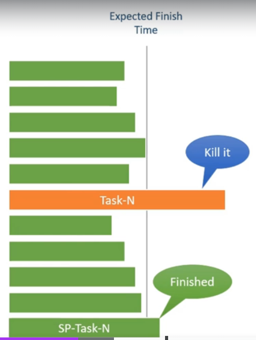
spark.speculation, false by default - example we have 10 tasks, and all of them complete under 2 seconds, but one of them takes 10 seconds
- spark will automatically identify the slow running tasks and run a duplicate copy of this task
- this way, whichever one of the two finishes faster is used by spark, and the other task is killed
- useful when for e.g. the original task was running slow due to a fault in the worker node that it was running on, which was causing it to be slow
- running speculative tasks does have overhead in terms of resources
- e.g. if there are data skews or out of memory issues in our application, spark would still run copies of this task (which too will run slow or maybe fail) without realizing that the root cause is actually the data / faulty configuration itself