Snowflake

we can create and run queries inside worksheets
we can see the snowflake_sample_data database by default with some sample data
1 select * from snowflake_sample_data.tpch_sf1.customer
we use snowflake’s virtual warehouses for mpp (massive parallel processing). this allows the query to be processed in parallel in small chunks
virtual warehouse sizes - xs (1 server), s (2 servers), m (4 servers),…4xl (128 servers)
when not in use, a warehouse can be suspended. configure this behavior automatically using auto suspend and auto resume
creating warehouses can be done by using the ui / even issuing sql statements in the worksheet
in the worksheet, we can set the context i.e. the current database, schema and warehouse or use commands like use warehouse or use database
multi clustering - when creating a warehouse, we can create it as a cluster and set the minimum and maximum number of warehouses allowed
i think multi clustering is an enterprise feature, i do not see the option for it in the ui
based on when load is high, this cluster will automatically add or remove warehouses for us (think asg in aws)
multi clustering is better for more number of queries, for more complex queries we might need to consider vertical scaling (increase size of warehouse)
notice difference between more number of queries vs more complex queries
so basically there is a queue of the queries, which gets assigned one by one to the warehouses
scaling policy - standard is the default whereas economy preserves the cost
- standard - add additional virtual warehouses if there is a task queued
- economy - add additional virtual warehouses if the estimated time for the current cluster is at least 6 minutes
optimize virtual warehouse usage -
- have dedicated virtual warehouses for different use cases since they have different workload types
- understand horizontal scaling (more concurrent queries) vs vertical scaling (more complex queries), and choose the right one based on use case
snowflake editions - standard, enterprise (has all features of standard with additional features like multi cluster warehouse, time travel upto 90 days as opposed to the 1 day inside standard, materialized views, etc), business critical (all features of enterprise with extended support etc) and virtual private (think dedicated hosts in aws ec2)
we are charged for storage (after compression) and compute (warehouse)
for storage, we have two options to choose between - on demand (pay for what you use) and capacity (pay upfront)
40$ per tb per month for on demand storage, 23$ per tb per month for capacity storage
for xs virtual warehouse, we consume 1 credit per hour consumed by second i.e. if we consume for half an hour, we use half a credit (minimum is one minute). number of credits consumed by a warehouse depends on size (1 credit per server, so medium would consume 4 credits per hour)
for virtual warehouse, we are charged in terms of credits. there is a conversion of credit and dollars associated with it. e.g. for cloud provider as aws and in the us-east-1 region - 2$ per credit for compute if using standard edition
methods of loading data in snowflake -
- bulk / batch loading - uses our compute. e.g. copy command
- continuous loading - doesn’t use our compute, serverless. e.g. snowpipe
stages - location from where data can be loaded
- external - maintains url, access credentials, etc. e.g. s3 buckets
- internal - local storage maintained by snowflake
note - there are costs considerations around data transfer when moving data from different regions or different clouds vs same cloud and same region

creating a stage -

  
create or replace database our_first_db;

create or replace database manage_db;
create or replace schema manage_db.external_stages;
  
create or replace file format manage_db.external_stages.csv_format
  type = csv field_delimiter = ',' skip_header = 1;

create or replace stage manage_db.external_stages.bucketsnowflakes3
  url = 's3://bucketsnowflakes3'; -- the bucket is unprotected

list @manage_db.external_stages.bucketsnowflakes3; -- lists files

create or replace table our_first_db.public.orders (
  order_id varchar(30),
  amount int,
  profit int,
  quantity int,
  category varchar(30),
  subcategory varchar(30)
);

copy into our_first_db.public.orders
  from @manage_db.external_stages.bucketsnowflakes3
  file_format = manage_db.external_stages.csv_format
  files = ('OrderDetails.csv');

doing some transformations before loading data -

  
copy into orders_ex (order_id, profit, profitable_flag) from (
  select
    s3.$1,
    s3.$2,
    iff(cast(s3.$3 as int) > 0, 'profitable', 'non profitable')
  from
    @manage_db.external_stages.bucketsnowflakes3 s3
)
file_format = manage_db.external_stages.csv_format
files = ('OrderDetails.csv');

instead of files where we specify the full names of the files in an array like structure, we can specify a regex to match file names using the pattern keyword
lets say we have a column of type integer in the create table statement, but the data in the csv inside s3 is bad and one of the rows in the csv has a string for the corresponding column. we can configure the behavior on encountering an error as follows -
1 2 3 -- ... files = ('OrderDetails_error.csv') on_error = skip_file;
the options for on_error are -
- abort_statement - the default. abort the copying and rollback the rows copied
- continue - skip the row where the error happened and continue the loading of data
- skip_file - skip the file where the error happened but continue loading other files. we can also configure the error limit per file in this case, e.g. skip_file_3 would mean skip the file if three or more errors happen (so skip_file actually means skip_file_1?)
before actually copying over the data, we can also do a dry run of the copy - this way we can know beforehand if the copying will go through without actually executing it. we configure this using validation_mode i.e. if we provide this option, the data is not actually copied
1 2 3 -- ... files = ('OrderDetails_error.csv') validation_mode = return_errors;
the two options are -
- return_errors - returns all errors if any during the execution of the entire thing. the output will contain the files where the error occurred, the row number, the reason of the error, etc
- return_n_rows - e.g. return_5_rows would mean perform the validation on only the first 5 rows, and if a failure occurs, throw the exception, and if no, return these 5 rows. note - the difference is this returns the processed rows while the above returns files where exceptions occurred
if column has type varchar(10) but the source csv column has values of larger lengths, the copy command will fail. we can prevent this failure by using truncatecolumns = true, so that columns with greater lengths are just truncated i.e. electronics will become electronic
by default, if we rerun the same copy command more than once, the rows will not be duplicated 🤯. we can change this behavior by providing force = true. note that this can lead to duplicates
to view the history of copy commands i.e. source stage, success vs failure count, etc, use -
1 select * from copy_db.information_schema.load_history;
note that the command above was for a single database. to view the same thing across databases, use the snowflake db
1 select * from snowflake.account_usage.load_history;
for loading unstructured data (e.g. json), we might not be able to load it directly like above i.e. csv rows were easily mapping one to one with table rows
so, we first load the json to a new table which has only one column of type variant

we then transform this data (e.g. flatten) to load into our own tables

  
create or replace stage manage_db.public.s3_json
    url = 's3://bucketsnowflake-jsondemo';

create or replace file format manage_db.public.json
    type = json;

create or replace table our_first_db.public.json_demo (
    raw_json variant
);

copy into our_first_db.public.json_demo
  from @manage_db.public.s3_json
  file_format = manage_db.public.json
  files = ('HR_data.json');

now, assume the json has the format as below -

  
{
  "city": "Louny",
  "first_name": "Dag",
  "gender": "Male",
  "id": 2,
  "job": {
    "salary": 43000,
    "title": "Clinical Specialist"
  },
  "last_name": "Croney",
  "prev_company": [
    "MacGyver, Kessler and Corwin",
    "Gerlach, Russel and Moen"
  ],
  "spoken_languages": [
    { "language": "Assamese", "level": "Basic" },
    { "language": "Papiamento", "level": "Expert" },
    { "language": "Telugu", "level": "Basic" }
  ]
}

we can for e.g. query city as follows -

  
select raw_json:city from our_first_db.public.json_demo;

recall raw_json was the variant column in our table. the output for e.g. of above would be a column containing cells of the format "Bakersfield". so, now to convert this to a string i.e. Bakersfield (without quotes), we can do the below -
1 select raw_json:city::string from our_first_db.public.json_demo;
for nested object e.g. refer job in the json, this would work -
1 raw_json:job.salary::int job_salary
for nested arrays e.g. refer languages in the json, this would work - note how we can only grab one language at a time since this is like one to many
1 raw_json:spoken_languages[0].language::string first_language
so, the above solution works for arrays if we are fine with introducing new columns like first_language, second_language, etc

but what if we want a table that is like if we had to perform a join between employee data and spoken languages -

  
select
    json_demo.raw_json:first_name::string first_name,
    flattened.value:language::string language
from
    our_first_db.public.json_demo json_demo,
    table(flatten(raw_json:spoken_languages)) flattened;

the output of this command would look like this -
first_name language
Portia Kazakh
Portia Lao
Dag Assamese
Dag Papiamento
Dag Telugu

first_name	language
Portia	Kazakh
Portia	Lao
Dag	Assamese
Dag	Papiamento
Dag	Telugu

now theoretically we could have done as below -

  
select
    raw_json:first_name::string first_name,
    raw_json:spoken_languages[0].language::string language
from
    our_first_db.public.json_demo
union all
select
    raw_json:first_name::string first_name,
    raw_json:spoken_languages[1].language::string language
from
    our_first_db.public.json_demo
union all
select
    raw_json:first_name::string first_name,
    raw_json:spoken_languages[2].language::string language
from
    our_first_db.public.json_demo;

notice the index of spoken_languages above. the downside is the output would be as follows i.e. there would be nulls inside the language row for people having less than three languages
first_name language
Portia Kazakh
Portia null
Portia null
Dag Assamese
Dag Papiamento
Dag Telugu
caching - snowflake has caching enabled by default, and it is cached for 24 hrs. to ensure this however, ensure that queries go on the same warehouse. this is why having dedicated virtual warehouses for dedicated groups can help
we can confirm if the cache was used by clicking on the query id - it shows table scan + aggregation for the first time, and shows query result reuse the second time onwards
clustering - snowflake creates cluster keys for columns to create micro partitions. this prevents full table scans
we can explicitly do clustering
- do it for columns which are usually used in where clauses
- do it for columns frequently used in joins (similar to above)
- avoid extremes -
  - not useful for columns which have too many unique values, e.g. id
  - not useful for columns which have too less unique values, e.g. gender
we can confirm clustering performance by clicking on the query id - it shows how many total partitions are there and how many partitions are used

first_name	language
Portia	Kazakh
Portia	null
Portia	null
Dag	Assamese
Dag	Papiamento
Dag	Telugu

connecting to s3 securely using integration objects -

create an iam role -
- select the trusted entity as the same account id in which this role is being created
- select the requires external id parameter and enter a random value here for now

above steps result in a trust policy like below. note that both values entered above are placeholders for now -

  
{
  "Version": "2012-10-17",
  "Statement": [
    {
      "Effect": "Allow",
      "Principal": {
        "AWS": "arn:aws:iam::8502136:root"
      },
      "Action": "sts:AssumeRole",
      "Condition": {
        "StringEquals": {
          "sts:ExternalId": "something-random"
        }
      }
    }
  ]
}

create an integration object inside snowflake -

  
create or replace storage integration snowflake_s3_demo
  type = external_stage
  storage_provider = s3
  enabled = true
  storage_aws_role_arn = 'arn:aws:iam::8502136:role/SnowflakeDemo'
  storage_allowed_locations = ('s3://snowflake-demo-3b98x97')

run describe storage integration snowflake_s3_demo and copy the values under STORAGE_AWS_IAM_USER_ARN and STORAGE_AWS_EXTERNAL_ID. replace the values in the trust policy for principal and external id with this

now, we can use the integration object when creating a stage -

  
create or replace stage manage_db.external_stages.csv_folder
  url = 's3://snowflake-demo-3x7'
  storage_integration = snowflake_s3_demo
  file_format = manage_db.file_formats.csv_fileformat

snowpipe - enables loading of data automatically when for e.g. a new file is added to the s3 bucket
snowpipe is serverless i.e. our compute is not used for this
this near realtime ability is achieved via s3 notifications sent to snowflake managed sqs queue

setting up a snowpipe -

create a pipe -

  
create pipe snowpipe_demo.public.s3
  auto_ingest = true as
      copy into snowpipe_demo.public.employee
          from @snowpipe_demo.public.s3_csv
          file_format = snowpipe_demo.public.csv
          pattern = '.*employee.*\.csv';

run the describe command to grab the queue arn - describe pipe snowpipe_demo.public.s3
set up event notification on the s3 bucket with this sqs arn as the destination

to view pipes, use show pipes or we can specify database as well using show pipes in database snowpipe_demo

to make changes to the pipe, pause it first -

  
alter pipe snowpipe_demo.public.s3 set pipe_execution_paused = true;

even if we want to make changes to data, e.g. to have existing files picked up the snowpipe, pause the snowpipe before running the copy command manually to load the data of existing files
time travel - e.g. we make an erroneous update like this -
1 update test set first_name = 'Shameek';

we can now go back in time to look at what the data looked like before the erroneous update -

  
-- go back a specific amount of seconds
select * from test at (offset => -60 * 2);
-- OR go back to a certain timestamp
alter session set timezone = 'UTC';
select current_timestamp;
select * from test at (timestamp => '2023-07-28 03:36:21.779'::timestamp);
-- OR before a certain query (the erroneous update in this case) was executed
select * from test before (statement => '01adeb9c-0604-af37-0000-007bd70792b5');

note - for the before statement query issued above, snowflake has a history of all queries executed which we can see in the ui

e.g. of restoring -

  
truncate table test;
insert into test (
  select * from test before (statement => '01adebc9-0604-af9c-0000-007bd707b315')
);

optionally, load the time traveled data into a backup table and then load it from here into the original table instead of loading the data into the original table directly as described above
if we accidentally drop a table / schema / database, we can run the undrop command, e.g. undrop table test to restore it
- optionally, if we accidentally run create or replace table test..., we can restore the test table before the replace command was executed by first renaming the current wrongly instantiated table, e.g. alter table test rename to test_aux, and then running the undrop command to restore the test table before the replace to our database
we can go back upto 90 days in editions enterprise and above, and upto 1 day in standard edition. however, the default is set to 1. therefore, we have to change the retention period manually to 90 days for editions other than standard -
1 alter table test_tt set data_retention_time_in_days = 2;
failsafe - protection of historical data in case of a disaster
the failsafe period starts after the time travel period ends
the failsafe period is for 7 days
this is not queryable / usable by front users like in time travel. the idea is to reach out to snowflake support after a disaster occurs to restore the table to a previous state
the failsafe period cannot be configured like time travel
table type - table type is a property of the table. the different table types are -
- permanent tables - this is the default. we have both time travel (0-90 days) and failsafe
- transient tables - we have time travel (0-1 day). but no failsafe
  1 create or replace transient table -- ...
- temporary - we have time travel (0-1 day) but no failsafe. note - this is only scoped to a session i.e. we loose this table when the session is closed / cannot view it from other sessions
  1 create or replace temporary table -- ...
the types above are not only scoped to a table, but to database / schemas as well
we would pay for additional storage for failsafe / time travel, so use transient tables for “reproducible” data like staging layer of warehouse?
zero copy cloning - when we use the clone command, the new table reuses the data and metadata of the older table. this way, it is cost efficient. the additional updates however do not effect one another
we can clone storage objects (databases, tables, schemas) and stages, file formats, tasks, etc

we can use time travel with cloning as well -

  
create table cloned
  clone source
  before (timestamp => ...)

swap table / schemas - swaps the underlying metadata and data as well

  
alter table swap_demo.public.development
  swap with swap_demo.public.production;

data sharing - data is not copied again, so it is automatically immediately up to date for the consumer
snowflake users it is shared with have to use their own compute resources for this

creating a share -

  
create or replace share orders_share;
grant usage on database data_share_demo to share orders_share;
grant usage on schema data_share_demo.public to share orders_share;
grant select on table data_share_demo.public.orders to share orders_share;

add account to share -

  
alter share orders_share add account = <<consumer-account>>;

create a database from the share inside the consumer account -

  
create database orders_db from share <<producer-account>>.orders_share;

now, the consumer can start consuming the data from this newly created database
till now, we assumed that the consumers have their own snowflake account when sharing data. non snowflake users can access shares via a reader account. however, our compute is used in this case

create a reader account

  
create managed account analytics
  admin_name = analytics
  admin_password = 'P4$$w0rcl'
  type = reader;

add the reader account to the share -

  
show managed accounts; -- use the value of "locator" for the value below
alter share orders_share add account = QBB35692;

in the reader account, create database from share -

  
show shares;
create database orders_db from share <<producer-account>>.orders_share;

create a virtual warehouse inside the reader account (looks like parent account virtual warehouses and reader account virtual warehouses are not exposed to each other?)

for granting select on all tables in a database / schema -

  
-- instead of
grant select on table data_share_demo.public.orders to share orders_share;
-- do
grant select on all tables in database data_share_demo to share orders_share;
-- or 
grant select on all tables in schema data_share_demo.public to share orders_share;

views - e.g. instead of sharing all data, we want to share some restricted data. we can do this via views. e.g. -

  
create or replace view data_share_demo.public.loan_payments_cpo as (
  select loan_id, principal
    from data_share_demo.public.loan_payments
    where loan_status = 'COLLECTION_PAIDOFF'
);

however, the issue with the above is for e.g. if we grant a role select on this view, and if a user with that role runs the command show views, they can view things like view definition. ideally, i would not have wanted to expose the fact that loan_status maintains an enum, since it is not even present in the projection clause of the view creation statement
creating a secure view - create or replace secure view...
note - we cannot use shares with normal views, we have to use secure views
data sampling - use a subset of dataset when for e.g. testing workflows out
two methods of sampling in snowflake -
- row or bernoulli method - every row is chosen with a probability of percentage p. so, it maybe more random since continuous rows are not chosen
  1 2 select * from snowflake_sample_data.tpcds_sf10tcl.customer_address sample row (1) seed (25); -- seed helps reproduce same results when using randomness
- block or system method - every block is chosen with a probability of percentage p. so, it maybe a bit more quicker, since it uses micro partitions
  1 2 select * from snowflake_sample_data.tpcds_sf10tcl.customer_address sample system (1) seed (25);

tasks - it stores an sql statement that can be scheduled to be executed at a certain time or interval

  
create or replace task task_db.public.customer_insert
  warehouse = compute_wh
  schedule = '1 minute'
  as
  insert into customers (created_date) values (current_timestamp);

notice how tasks use our compute unlike snowpipe, materialized views, etc?
on running show tasks, feels like tasks are suspended by default. so, run the following -
1 alter task task_db.public.customer_insert resume;
for crons, - schedule = 'USING CRON * * * * * UTC'
tree of tasks - a root task, which can then have children (multiple levels are allowed). one child task can have one parent task, but one parent task can have multiple children. when declaring a child task, instead of schedule, we use after task_db.public.parent_task
note - i think the parent task needs to be suspended first i.e. we first suspend the parent task, create and resume the child task and then finally resume the parent task, else we get an error. even as a best practice that feels right
getting execution history of tasks like errors, completion time, etc. it also has records for the next queued execution
1 select * from table(task_db.information_schema.task_history(task_name => 'customer_insert'));
tasks can also have a when clause, and the task is executed only if the condition evaluates to true, else the task is skipped
streams - helps with cdc (change data capture) to capture the delta (changes) of the source data. so, streams help capture dml (i.e. crud) changes
we only pay for the storage of metadata columns of the stream that helps determine whether the row was deleted, updated, etc. the rows in streams reference the original source for the actual data

create a stream -

  
create or replace stream streams_demo.public.sales_raw_stream
    on table streams_demo.public.sales_raw;

we can run select on the stream table just like we would on a normal table
1 select * from streams_demo.public.sales_raw_stream;
the stream has three additional columns - METADATA$ACTION, METADATA$ISUPDATE, METADATA$ROW_ID
once we process the stream, the data in the stream is deleted. it feels like stream is like an “auto generated temporary staging layer” of the warehouse. e.g. if i insert into a table by running a select on the stream table, the stream table clears up
an update corresponds to two rows in streams - an insert and a delete for METADATA$ACTION, and true for METADATA$ISUPDATE in both rows. so, METADATA$ACTION is always either insert or delete, and we need to determine if the change is due to an update using METADATA$ISUPDATE

e.g. of using streams - imagine store is a static reference table. we want to process the changes in sales table to a table used for analytics, that is like a join between sales and store tables. so, we can assume that for every record in the sales table, there would be a record in this sales analytics table, with added information about the store. so, the stream is needed for the sales table, and not the store table, and we update the final table used for analytics by joining the sales stream table and store reference table

  
create or replace stream streams_demo.public.sales_raw_stream
  on table streams_demo.public.sales_raw;

merge into streams_demo.public.sales_final sf
using (
    select sa.*, st.employees, st.location
    from streams_demo.public.sales_raw_stream sa
    join streams_demo.public.store_raw st
    on sa.store_id = st.store_id
) src
on src.id = sf.id
    when
        matched
        and src.METADATA$ACTION = 'DELETE'
        and not src.METADATA$ISUPDATE
        then delete
    when
        matched
        and src.METADATA$ACTION = 'INSERT'
        and src.METADATA$ISUPDATE
        then update set
            sf.product = src.product,
            sf.price = src.price,
            sf.amount = src.amount,
            sf.store_id = src.store_id,
            sf.location = src.location,
            sf.employees = src.employees
    when
        not matched
        and src.METADATA$ACTION = 'INSERT'
        and not src.METADATA$ISUPDATE
        then insert values (
          src.id,
          src.product,
          src.price,
          src.amount,
          src.store_id,
          src.location,
          src.employees
        );       

we can use streams in the when clause of tasks! so, we can pretty much build an entire etl pipeline just using snowflake -
1 2 when system$stream_has_data('stream-name') as -- the entire sql for stream processing defined above
stream types - standard and append-only. append-only captures only inserts while standard captures inserts, updates and deletes. default is standard as seen above
change tracking - tables have a change tracking property. we can set it to true as follows -
1 alter table names set change_tracking = true;
now, with change tracking enabled, we can basically see the changes in a table in the same format as we saw in streams -
1 2 3 select * from names changes (information => default) at (offset => -240);
my understanding - the difference is that unlike streams, this does not get deleted. its almost like we have a rolling window of cdc until the time travel / retention period
again - notice the use of default in the changes clause above. we can also use append_only instead
materialized view - if we run an expensive query frequently, it can lead to bad user experience. so, we can instead use materialized views
1 2 create or replace materialized view orders_mv as -- ...
so, materialized views are updated automatically when its base tables are updated. this updating is maintained by snowflake itself. when we query using materialized view, data is always current
this means that if the materialized view has not been updated completely by the time we initiate a query, snowflake will use the up to date portions of the materialized view and fetch the remaining data from the base tables
since background services of snowflake are being used for updating materialized views, it adds to the cost independent of our virtual warehouses
use materialized views if data is not changing frequently and view computation is expensive. if data is changing frequently, use change tracking / streams + tasks
has a lot of limitations i think 😭 - joins, some aggregation functions, having clause, etc are not supported at the time of writing

dynamic data masking - returns masked results for security purpose, e.g. pii (personally identifiable information)

  
create or replace masking policy phone
  as (val varchar) returns varchar -> 
    case
      when current_role() in ('ACCOUNTADMIN') then val
      else '#####'
    end;
  
alter table customers
  modify column phone_number
  set masking policy phone;

some more masking policy examples -
- we just want to see the domain of the emails -
  1 when current_role() not in ('ACCOUNTADMIN') then regexp_replace(val, '+\@', '****@')
- we want to be able to do comparisons, e.g. we want to join by name, but we do not want to allow seeing of the names. we can use sha2(val), so that while users see an encrypted value, it is a consistent hash, so running it on the same value will produce the same result

Access Management

rbac (role based access control) i.e. privileges are assigned to roles, which are inturn assigned to users
in snowflake we have dac (discretionary access control) i.e. every object has an owner, who can grant access to that resource. so, all objects have an owner, which is a role, and this role has all privileges on that object by default. the objects on which we can grant privileges are also called securable objects, e.g. warehouses, databases, tables, etc
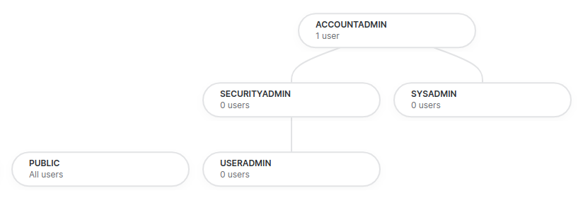
role hierarchy - the parent role will automatically have the privileges of all of its child roles
my understanding
- a user can have multiple roles
- the public role is assigned to all new users by default
- the default role is the one that determines what role to use when for e.g. a new worksheet is opened by the user, or maybe like when no role is specified
- for all roles to be used, set secondary role to all. e.g. we have a system account, which has warehouse access via a different role, and access to tables via yet another role. we cannot specify both roles in for e.g. the jdbc url. so, we can instead set the secondary role to all for permissions from all roles to kick in for a user anytime the user makes a query

system defined roles -

account admin -
- the top level role
- can manage things like reader accounts
- avoid using this, and users using this should use mfa
- do not create objects using this, as otherwise we would have to manually add privileges to users that need it (it is at the top of hierarchy so no role inherits “from” it)
- only account admin can view things like usage / billing information

security admin -

can manage any object grant globally - my doubt - does this mean it can do this for objects that it (or its nested children) do not own as well?
can be used to create and manage roles but thats usually done by useradmin?

example - (note the hierarchy i.e. sales_user is a child of sales_admin, which is inturn a child of sysadmin. this is a best practice)

  
create or replace role sales_admin;
create or replace role sales_user;

grant role sales_user to role sales_admin;
grant role sales_admin to role sysadmin;

create or replace user simon_sales_user
    password = 'p@$$worcl'
    default_role = sales_user;
grant role sales_user to user simon_sales_user;

create or replace user olivia_sales_admin
    password = 'p@$$worcl'
    default_role = sales_admin;
grant role sales_admin to user olivia_sales_admin;

sysadmin -
- create warehouses, databases, etc
- custom roles should be attached to sysadmin as a best practice. this way, the objects created by these custom roles can be managed by sysadmin. otherwise, this would not be possible
- example - we run the below from inside sysadmin. despite us granting ownership to sales_admin, sysadmin can still perform all the operations on these objects since sysadmin inherits permissions from sales_admin. refer above, this setup was basically done by security admin
  1 2 3 create or replace database sales_db; grant ownership on database sales_db to role sales_admin; grant ownership on schema sales_db.public to role sales_admin;
- now, from inside sales_admin, we can run the below -
  1 2 3 grant usage on database sales_db to role sales_user; grant usage on schema sales_db.public to role sales_user; grant select on table sales_db.public.customers to role sales_user;
useradmin -
- used to create / manage users and roles
- unlike securityadmin, it does not have ability to grant privileges to all objects, only on objects that it owns
public role
- every user is granted this role by default

Snowflake Architecture

query processing -
- uses virtual warehouses
- each virtual warehouse is a mpp cluster of compute nodes
- its size (ranging from xs to 6xl) governs the compute, memory, cpu, etc it will have
- each increase in size almost doubles the compute power
- account for most of the credit consumption
- scale statically or dynamically using multi cluster warehouses
storage -
- store in columnar format
- use compression when storing to reduce size by 3-5 times
- cost of storage is typically negligible
cloud services -
- brain of the platform
- login, query dispatch, query optimization, key management for encryption, etc
- runs on compute managed by snowflake
snowflake is saas - all three layers of snowflake run on selected cloud provider - aws, gcp, azure
we also need to select the region based on the cloud provider we choose
choice of these influence our cost of snowflake infrastructure, data egress costs, etc

Snowflake Costs

we are charged using credits. it is a unit of measure which is consumed when we use snowflake resources
our cost = compute + storage + data transfer + cloud services + serverless
compute cost -
- three factors - number of virtual warehouses, size of virtual warehouses and how long they run
- we are charged even if the warehouse is idle
- we are not charged when the warehouse is suspended - so, guard rails like auto suspend are important to save costs
- we are charged for a minimum of 60 seconds, and every second the warehouse is not suspended from then
storage cost -
- the default compression leads to reduced costs
- calculated based on average terabytes used daily over the month
- three main costs - data in stages, data stored in tables, features like failsafe and time travel
- also influenced by type of storage - on demand vs capacity - capacity is pre purchased, thus leading to much lesser costs
data transfer cost -
- cost is incurred if data is transferred
  - from one region to another
  - from one cloud to another
- a data egress charge is applied by the cloud providers - data ingress is typically free
- charge is per byte
cloud services cost -
- collection of services like metadata management, query processing and optimization, authentication, etc
- charged if consumption exceeds 10% of total compute resources
- it is calculated on a daily basis
serverless cost -
- uses compute managed by snowflake
- snowflake automatically decides the ideal size and scales its compute automatically based on it
- cost is per second per core
- each serverless feature appears as a different line item in the bill
- costs incurred by some of the different serverless features are described below
- snowpipe - loads data from stages to tables automatically
  - compute costs
  - costs for number of files processed
- materialized views -
  - cost of compute used for the pre computation using the background process
  - storage costs
- database replication -
  - costs of compute for the synchronization
  - cost of data transfer from one region to another
  - cost of storage used by target database
- search optimization - used when selective filters used repeatedly only return a small amount of rows from the huge data. an “access path structure” is maintained for the efficient querying
  - storage costs for maintaining the structure
  - compute costs for maintaining the structure
- clustering - snowflake stores data in a sorted way to improve query performance. can be automatic or based on columns we specify
  - costs for initial clustering
  - costs for reclustering - reclustering happens periodically when our dml causes the clustering to fall out of sync significantly

Cost Governance Framework

visibility - understand, attribute and monitor the spend. e.g. dashboards, tagging, resource monitors. TODO - links
control - limit and control the spend. e.g. TODO - links
optimization - optimize the spend. e.g. TODO - links

Dashboards

Consumption Dashboard

admin -> cost management -> consumption will show credit consumption

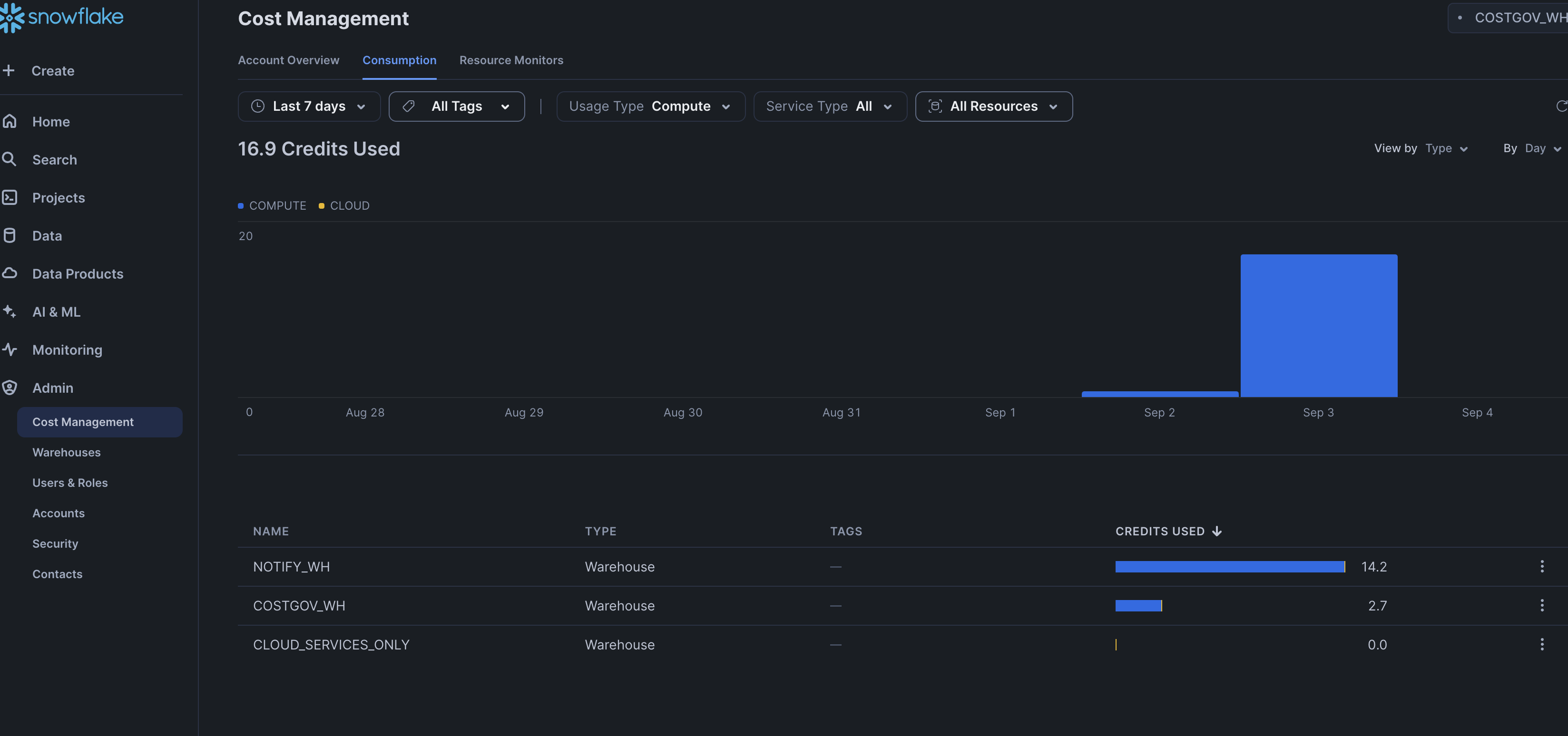
usage type - select one of
- compute - guessing compute includes all three - user managed warehouses, serverless features and cloud services
- storage
- data transfer
in this dashboard, we can change the grouping (by service, by resource, etc), change the date range (last 7 days, last 28 days, etc), and so on

Custom Dashboard 1

based on how we group, we either see for e.g. costs incurred by different database, or costs incurred by failsafe vs database
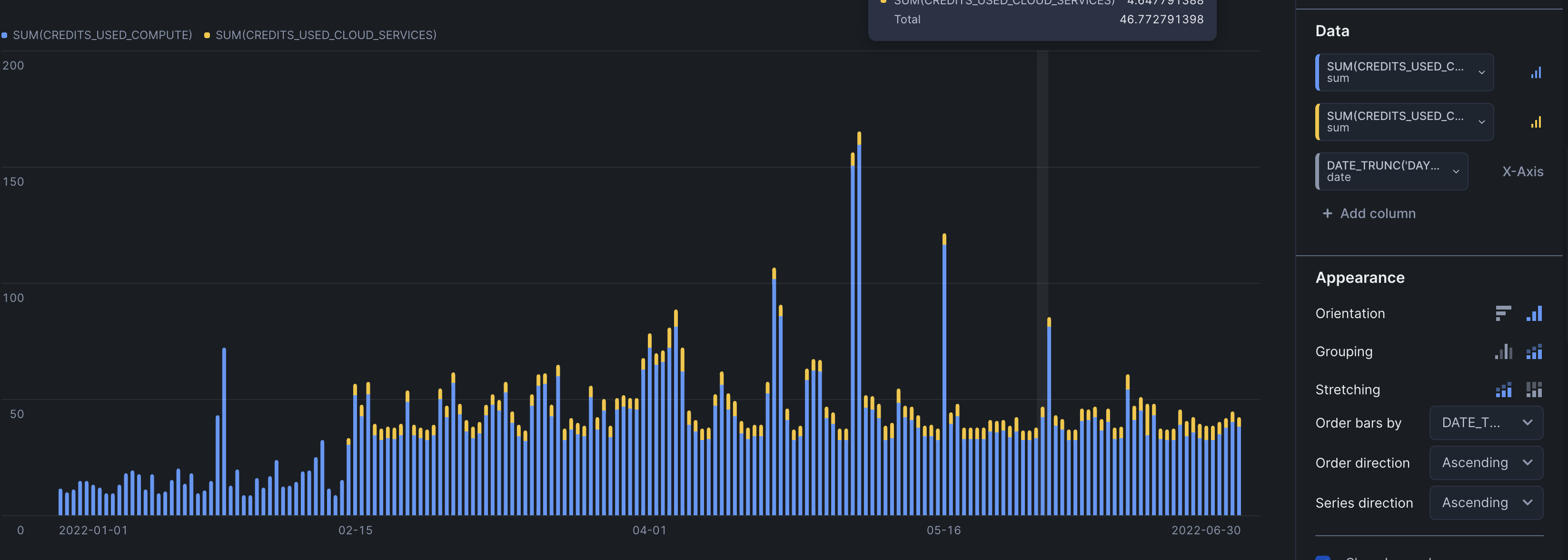
there is a read only database called snowflake, with a schema called account_usage. it has several views which contain data about the historical usage and costs associated with it

warehouse_metering_history - per virtual warehouse consumption at an hourly level

  
select
    date_trunc('day', start_time),
    credits_used,
    credits_used_cloud_services,
    credits_used_compute
from
    snowflake_finance.account_usage.warehouse_metering_history
where
    start_time = :daterange

i guess credits_used = credits_used_cloud_services + credits_used_compute
using the daterange filter helps us pick custom date ranges from the date picker
now, when creating a bar chart, values in x axis are unique. therefore, we need to select an aggregation type for values in y axis. we use sum

my understanding - right now, we fetch all records in the given range, and rely on our tile configuration capabilities. we can rely on the query to do that as well

  
select
    date_trunc('day', start_time),
    sum(credits_used),
    sum(credits_used_cloud_services),
    sum(credits_used_compute)
from
    snowflake_finance.account_usage.warehouse_metering_history
where
    start_time = :daterange
group by
    1

note - in our tile configuration, we will still have to provide the aggregation function etc, since the tile does not understand we have already ensured unique values for our x axis
orientation can be vertical or horizontal
grouping can be grouped (one beside another) or stacked (one on top of another)
we can also identify the direction of ordering etc

till now, whatever we saw till now tells us credits used by virtual warehouses. these include -
- virtual warehouses managed by us
- virtual warehouses managed y cloud services
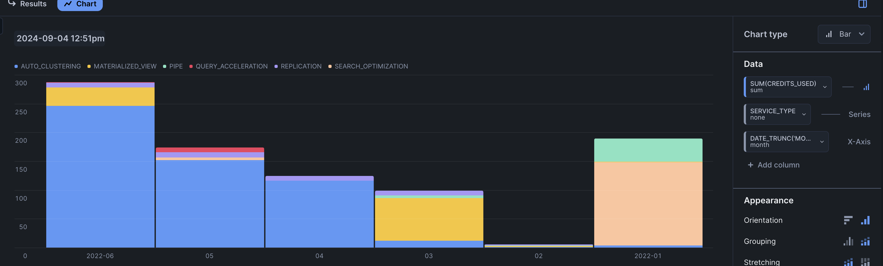
we can also monitor credits used by serverless compute. recall how it is broken down by services

so, we use metering_history for this, and filter out the rows for virtual warehouses

  
select
    date_trunc('month', start_time),
    service_type,
    sum(credits_used)
from
    snowflake_marketing.account_usage.metering_history
where
    start_time = :daterange
    and service_type != 'WAREHOUSE_METERING'
group by
    1, 2

Custom Dashboard 2

we can for e.g. budget 18,000 credits for snowflake for a year - this means 18,000 / 12 = 1500 credits per month
we can also establish a baseline - forecast based on usage values over previous months

note - while we are calculating these values in our dashboard, we would ideally store it in a table and query it for our tile

  
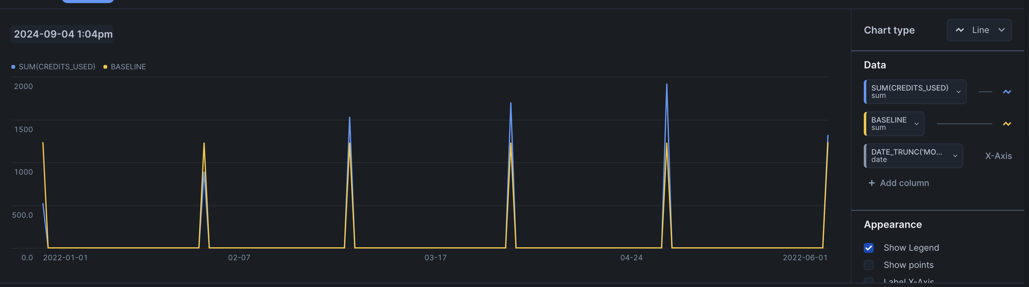
set baseline_start_date = '2021-09-01';
set baseline_end_date = '2021-12-31';
  
set baseline = (
    select
        round(sum(credits_used), 2) / 4
    from
        snowflake_finance.account_usage.metering_history
    where
        start_time between $baseline_start_date and $baseline_end_date
);

now, we can create the chart for the expected / baseline / budgeted amount vs the actual consumed credits -

  
select
    date_trunc('month', start_time),
    sum(credits_used),
    $baseline baseline
from
    snowflake_finance.account_usage.metering_history
where
    start_time = :daterange
group by
    1

the chart looks as follows -
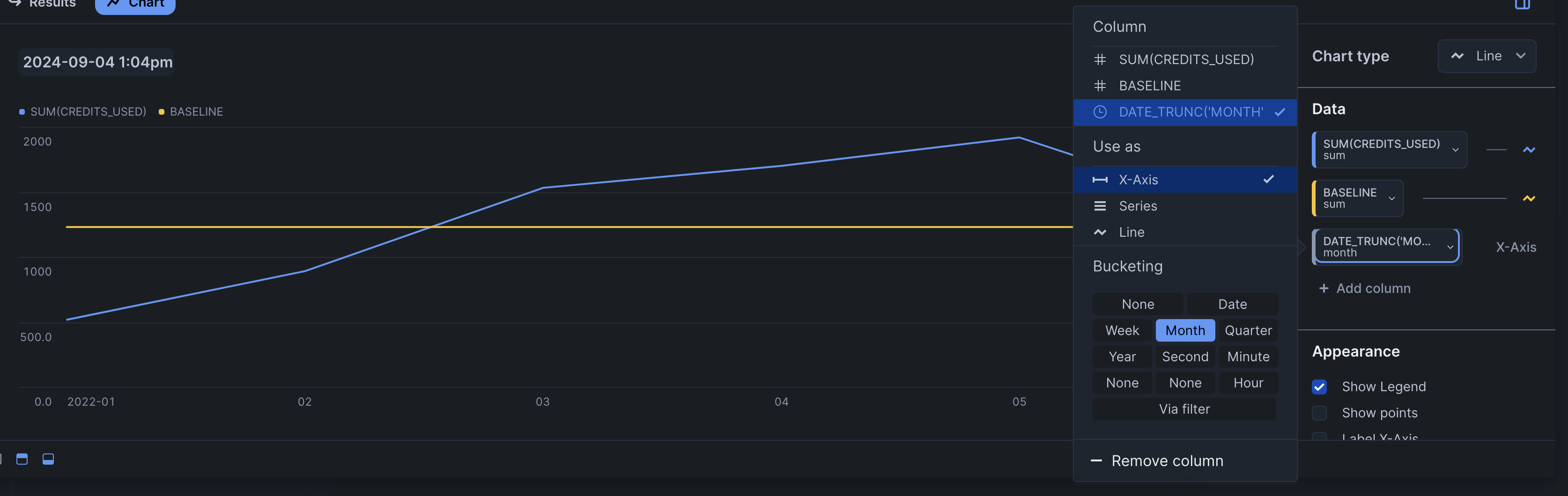
issue - the chart is not bucketed for the x axis properly. choose bucketing as month

final improvement - our budgeted amount adds up - e.g. if we budgeted 1500 credits, it adds up over the month, it does not stay at a constant. so does our consumption. such calculations are also called year to date i believe

  
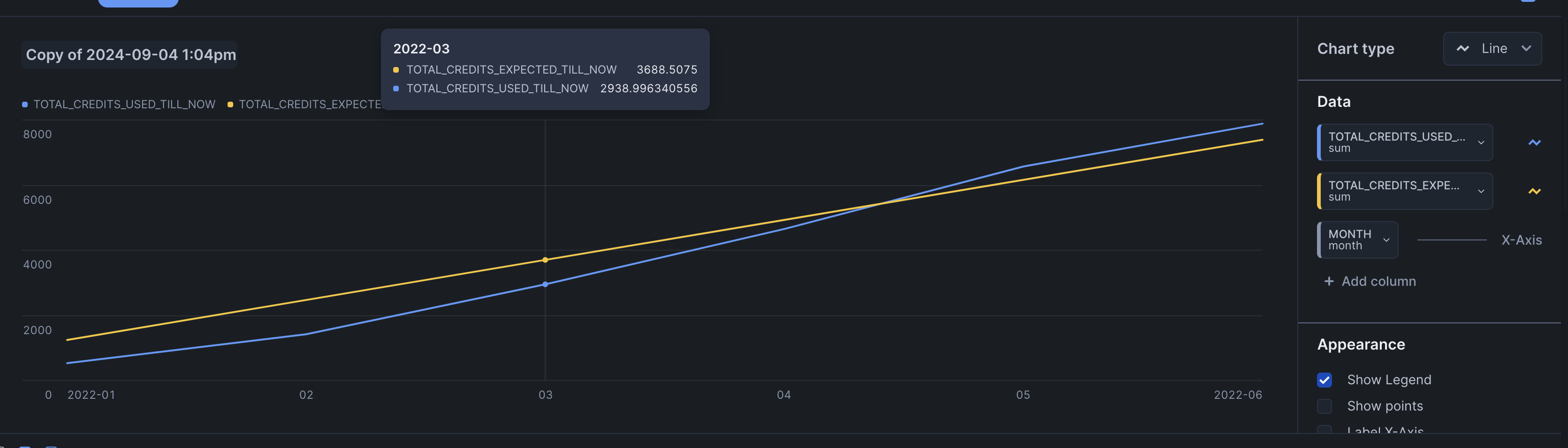
with usage as (
    select
        date_trunc('month', start_time) month,
        sum(credits_used) credits_used,
        $baseline credits_expected
    from
        snowflake_finance.account_usage.metering_history
    where
        start_time = :daterange
    group by
        1
)
select
    month,
    sum(credits_used) over (order by month) total_credits_used_till_now,
    sum(credits_expected) over (order by month) total_credits_expected_till_now
from
    usage

so, we use window functions. my understanding - we only need cumulative, and so we use the sum function and order by month. we do need to partition using a column

Warehouse Utilization

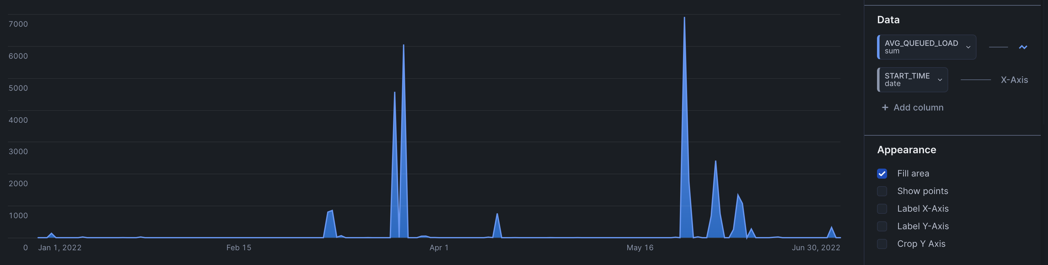
track this using warehouse_load_history
avg_queued_load - average number of queries queued -
- warehouse was overloaded - evaluate using multi cluster warehouses
- this might also indicate that our warehouses have been spinning up and down frequently, thus being unable to cache data efficiently and therefore return results quickly. solution - evaluate settings for auto suspend and auto resume, ensure that the same warehouse is used for the same query, etc
1 2 3 4 5 6 7 select start_time, avg_queued_load from snowflake_marketing.account_usage.warehouse_load_history where start_time = :daterange

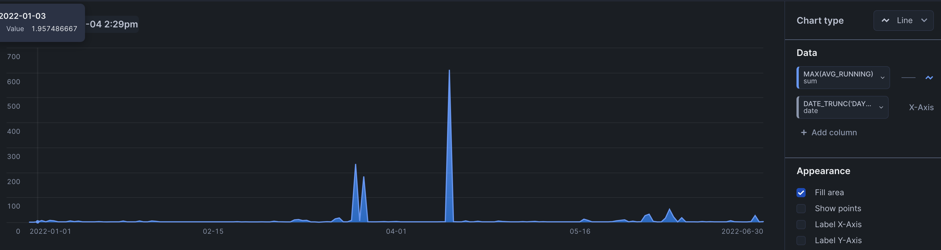
avg_running - average number of queries executed
- recall that a single virtual warehouse is a cluster of compute nodes
- consolidation - if we have two bi applications that rarely use a warehouse concurrently, we can use the same warehouse for both of the applications to reduce costs
1 2 3 4 5 6 7 8 9 select date_trunc('day', start_time), max(avg_running) from snowflake_marketing.account_usage.warehouse_load_history where start_time = :daterange group by 1

Object Tagging

we need to bucket costs by attributing it with tags
chargeback model - apply costs of it services to the business team that uses them

creating tags and adding it to objects -

  
create tag "635de402978_tag" comment = 'product name';
  
alter table product2_tbla set tag "635de402978_tag" = '6b27e2dc9_value';

select * from snowflake.account_usage.tag_references;

querying using tags -

  
use database snowflake;
use schema account_usage;
  
select
    tag_references.tag_value,
    sum(table_storage_metrics.active_bytes) total_bytes,
    count(*) total_tables
from
    tag_references
    left join table_storage_metrics on table_storage_metrics.id = tag_references.object_id
where
    tag_references.domain = 'TABLE'
    and tag_references.tag_name = '635de402978_TAG'
group by
    tag_references.tag_value

below points are my understanding -
- the table tag_references in snowflake.account_usage will give us what object is tagged with what
- we can now perform a join with tables like table_storage_metrics
- we perform a join - maybe because objects to tags is one to many. maybe a left join is used to report 0 for business units with no objects
- we filter for only objects of type table and the tag we are looking to report on - e.g. product name in our case
- we group using the distinct tag values, and perform an aggregation on the active bytes

Query Tagging

object tagging allows us to tag objects like databases, warehouses, etc
query tagging allows us to tag queries
while we do not have access to the credits consumed for these queries
we do have access to things like partitions scanned, average time elapsed, etc
e.g. tag all the queries in a dashboard to efficiently get analytics around the queries in it
1 alter session set query_tag = 'xyz';

running analysis on this -

  
select
    count(*) total_selects,
    avg(total_elapsed_time) avg_run_time,
    date_trunc('day', start_time) date
from
    snowflake_marketing.account_usage.query_history
where
    start_time = :daterange
    and query_tag = 'query tag f493ed5ca5aecf3b77b2c154cdc0b708'
    and query_type = 'SELECT'
group by
    date

Resource Monitors

resource monitors - warehouses can be assigned resource monitors
we can define a limit on the number of credits consumed - when this limit is reached, we can be notified
notification works on both user managed warehouses and warehouses managed by cloud services

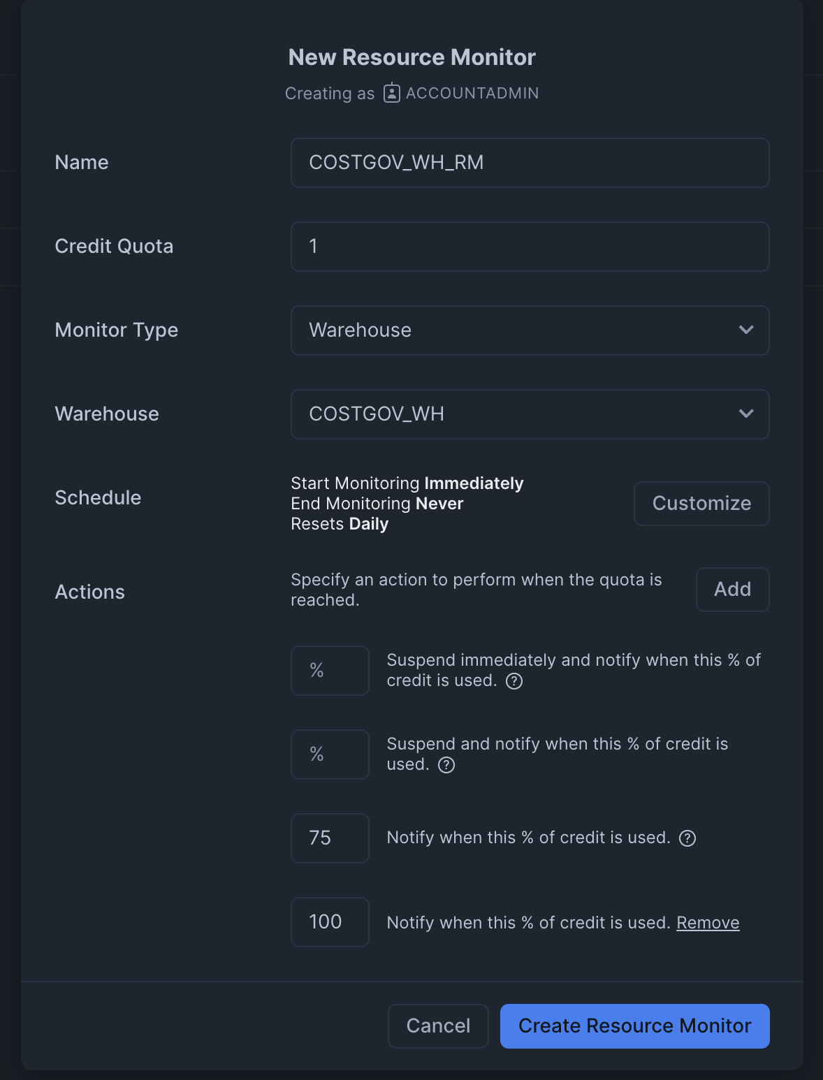
in the above resource monitor, we -
- set credit quota to 1
- monitor type - we can monitor the entire account or only a specific warehouse
- select the warehouse to monitor - a warehouse can have only one resource monitor, but the same resource monitor can be used for multiple warehouses
- start monitoring immediately, and never stop monitoring
- reset the monitor daily - it starts tracking from 0 again
- notify when 75% and 100% of the quota is consumed

i ran this statement to modify the users to be notified -

  
alter resource monitor costgov_wh_rm set notify_users = ('COSTGOV_LEARNER');

finally, on reaching the consumption, i get an email as follows -

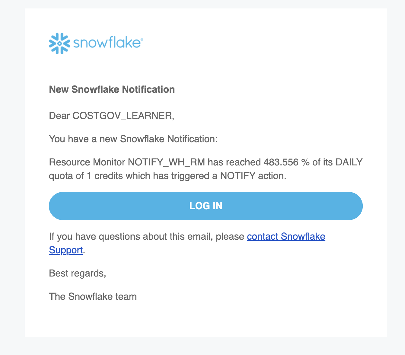
note - i also had to enable receiving notifications in my profile -

till now, we saw the visibility aspect of resource monitors, now we look at its control aspect
we can only suspend user managed warehouses, not ones managed by cloud services
we can choose to suspend either after running queries complete, or after cancelling all running queries

Control Strategies

virtual warehouses can be single cluster or multi cluster
changing warehouse size helps with vertical scaling (scaling up) i.e. processing more complex queries
using multi cluster warehouse helps with horizontal scaling (scaling out) i.e. processing more concurrent queries
some features of warehouses include to control spend include -
- auto suspend - automatically suspend warehouses if there is no activity
- auto resume - automatically restart the warehouse when there are new queries
- auto scaling - start warehouses dynamically if queries are queued. bring them down when queue becomes empty. there are two scaling policies - standard and economic. first prefers starting additional warehouses, while the second prefers conserving credits
statement_queued_timeout_in_seconds - statements are dropped if queued for longer than this. default is 0 i.e. never dropped
statement_timeout_in_seconds - statements are cancelled if they run for longer than this. default is 48hrs

Snowflake

Snowflake

Access Management

Snowflake Architecture

Snowflake Costs

Cost Governance Framework

Dashboards

Consumption Dashboard

Custom Dashboard 1

Custom Dashboard 2

Warehouse Utilization

Object Tagging

Query Tagging

Resource Monitors

Control Strategies

Further Reading

DBT

Spark Advanced

Python Data Analysis