Iceberg

Introduction

• rdbms are good for oltp workloads, not olap workloads involving aggregate queries on a large number of records
• components of an olap system - storage, file format, table format, storage engine, catalog, compute engine
• “storage” -
  • should handle storing “large” amounts of data
  • options - local filesystem, das (directly attached storage), distributed file system (hdfs), object storage (s3)
• “file format” -
  • affects how raw data is organized
  • this in turn affects compression, data structure, performance, etc
  • categories - structured, semi structured, unstructured
  • types - row oriented (csv and apache avro) or column oriented (apache parquet and apache orc)
• “table format” -
  • how data files are laid out
  • abstract away complexities of dml, maintaining acid guarantees, etc
• “storage engine” -
  • interacts with the storage
  • maintaining indices, physical optimization of the data, etc
• “catalog” -
  • compute engines use the catalog
  • it helps identify the existence of a table, its name, schema, where it is stored in the storage layer, etc
• “compute engine” -
  • deal with the massive amounts of data
  • make use of mpp (massive parallel processing)
• now, data warehouses were the initial olap systems. cons -
  • all these components described above were proprietary / coupled to the warehouse. this is a “closed form” of architecture. so, all kinds of bi and ml workloads would be bound to this platform
  • storage and compute in earlier warehouses were coupled, thus making them difficult to scale
  • comparatively costly
  • only meant for structured data, but unstructured data like text, images, etc have a lot of valuable insights
  • not optimized for ml based tasks
• lake evolution -
  • originally, hadoop was used to store huge amounts of data - both structured and unstructured, and it works for ml workloads too
  • map reduce was used as the analytics framework on top of it
  • eventually, people used hive to query using sql instead of complex java code
  • this was because the “hive table format”, could recognize a directory and the files inside it as a table
  • eventually, map reduce fell out in favor of spark, presto, dremio, etc
  • similarly, hdfs fell out in favor of s3, azure blob, etc
  • however, the hive table format still stayed
• notice how the lake architecture addresses all the cons of the data warehouses we saw above. however, the cons of lake architecture are as follows -
  • the lake architecture is not as optimized as warehouses in terms of performance
  • lake architecture does not have acid guarantees for updates
  • unlike data warehouses, there is significant maintenance overhead in terms of tools etc
  • there is no “storage engine” - the “compute engine” directly writes data, which is never revisited or optimized, unless the entire table / partition is rewritten
  • while engines like spark etc can perform reads efficiently, the writes are still inefficient
• so, clearly, we need benefits of both worlds. that is why lakehouse was born. it brings data warehouse like functionality to lake
• “hive table format” - a directory (or prefix in object storage) represents a table. subdirectories within it represent “partitions”
• all the metadata, as in what directory represents what table is tracked inside the “hive metastore”
• hive table format pros -
  • efficient querying using bucketing / partitioning to avoid full table scans
  • supports multiple file formats like parquet etc
  • using swaps of directories, it supported atomic changes to a partition
• hive table format cons -
  • hive metastore only allows for atomic changes to a partition, not individual files
  • similarly, it does not allow for atomic updates to multiple partitions
  • the hive table format requires frequent listing of files and directories. listing all the files and nested directory structure every time is inefficient in the query planning phase
  • it is not optimized for object storage - if a partition has all the files, the same prefix of the object storage gets used. there is typically throttling limits on a prefix, thus resulting in performance issues
  • table statistics are performed asynchronously, and often stale
  • e.g. assume the table is partitioned using month. if a user performs filtering using the timestamp column without mentioning the month column in the filter clause, a full table scan is done
  • if the partitioning scheme of a table changes, the whole table would need to be rewritten, which can be very expensive for huge datasets
• apache iceberg, apache hudi and delta lake are all “table formats”
• these table formats, unlike hive table format, used files instead of directories for granularity. this difference addresses all the cons mentioned about hive like acid guarantees across multiple files / partitions, efficient query planning, etc

Apache Iceberg Features

• “acid transactions” -
  • it works with multiple readers and writers
  • it uses “optimistic concurrency control” to minimize locking and improve performance
  • acid guarantees are ensured using the catalog
• “partition evolution” -
  • with hive etc, a change in partitioning scheme would require rewriting of the whole table, which can be very expensive for big tables
  • with iceberg, we can change the partitioning midway, e.g. from month to day of timestamp. since this is maintained in the “metadata file” described here, iceberg can handle it easily
• “hidden partitioning” -
  • e.g. assume we have a timestamp column
  • in hive etc, if we want to partition by day, month, etc, we would create new columns
  • this means that if the user filters using the original timestamp only, the partition pruning is not applied
  • people should not have to care how a table is partitioned
  • in iceberg, we can apply transforms like truncate, bucket, year, month, etc to the column to specify the partitioning scheme
  • this way, we do not have to maintain extra columns, and the filtering works as expected as well
• “row level table operations” -
  • two strategies to handle writes - cow (copy on writes) and mor (merge on reads)
  • “copy on write” - the entire data file is rewritten, with the row level changes
  • “merge on read” - the new file only contains the changes. all this is reconciled on reading. this helps speed up heavy update and delete workloads, at the cost of slowing down reads
• “immutable snapshots” -
  • iceberg uses immutable snapshots
  • advantage 1 - this allows us to “time travel” i.e. query the table in a point of time
  • advantage 2 - this allows us to perform “rollbacks” in case of mistakes

Iceberg Structure

Data Layer

• this layer provides the result of queries
  • exception - max of a column can be responded by metadata layer sometimes
• can be implemented using a distributed file system like hdfs, or object storage like s3
• flexibility of file formats
  • use parquet - for large scale olap workloads
  • use avro - for low latency stream analytics
• parquet file structure -
  • each parquet file has a set of rows called “row group”
  • it is broken down into “columns” (recall - parquet is column oriented)
  • columns are broken into subsets called “pages”
  • so, each page = values for a column for a set of rows
  • now, each of these pages can be read independently and in parallel
  • additionally, statistics like minimum and maximum are stored, that can help prune the data
• all the data is stored in “data files” of the data layer
• the data layer also has “delete files”
• note - delete files only apply to the “merge on read” strategy, not “copy on write”
• there are also two strategies of deletes - “positional deletes” and “equality deletes”
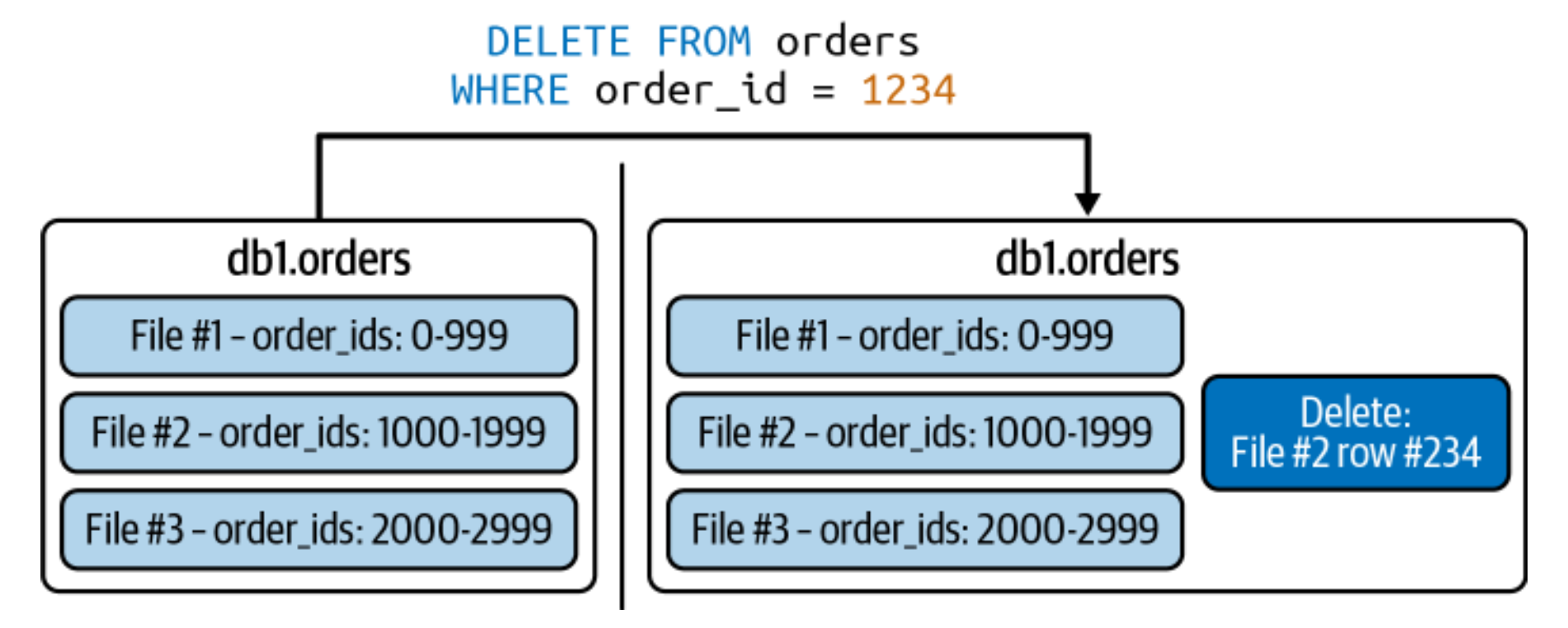
• “positional deletes” -
  • identify the rows to delete using their exact position in the dataset
  • the delete file can point to the exact data file and the line number in that file containing that row
  • e.g. the dataset is sorted using order_id, and we delete order_id = 1234. below is the before and after. look at the contents of the delete file

  

• “equality deletes” -
  • identify the rows to delete using one or more fields
  • in this case, there is no reference to the data files actually containing the record
  • what if a record is deleted and then added back? this scenario is handled using “sequence numbers”
  • the original data file will have a sequence number of 1, the delete file a sequence number of 2, and the final data file will have a sequence number of 3
  • when the engine reads the files, it will know to apply the operation of sequence number 2 only to files having a sequence number less than 2

Metadata Layer

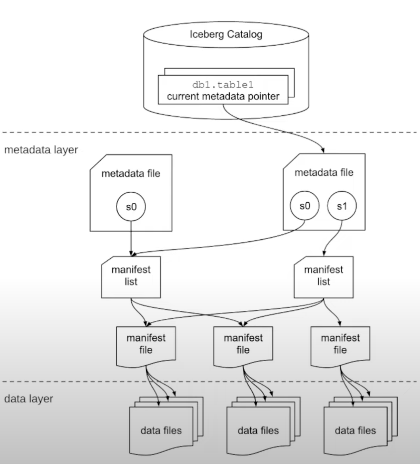
• “manifest file” -
  • contain list of datafile’s location
  • also contains datafile’s metadata like minimum and maximum. this helps with efficient query planning
  • the writer responsible for writing its set of files itself writes these statistics of maximum, record count, etc as well. doing this is much more easy for the writer as an additional step
  • this approach is much more efficient than hive. in hive, this is done by separate asynchronous jobs. this meant stale statistics. they were also much more heavy, since these jobs would run on entire partitions
• “manifest list” -
  • represents a snapshot
  • points to a list of manifest files. contains an array of objects, where each object represents a manifest file
  • it also contains stats around those manifest files, which helps for efficient query planning
• “metadata file” -
  • contains information about the table schema, partition information, list of manifest files and which manifest file is the current one
  • every time a change is made to a table, a new metadata file is created and registered with the catalog
  • this helps handle concurrent writes

Puffin Files

• helps enhance results of specific types of queries
• e.g. we want the unique people who placed an order in the last 30 days
• the statistics in the datafiles can help
• despite the pruning, we would still have to go through all the orders in the last 30 days
• “puffin files” can store statistics to help run queries like these quicker
• the only supported type currently is the “theta sketch” from the “apache data sketches” library
• this helps compute the approximate distinct values

Catalog

• it contains a table to metadata file pointer
• this helps the compute engine etc know how to interact with a particular table amidst thousands of tables
• it needs to support “atomic operations” - this helps handle concurrent writers
• a writer creates the new manifest file, and before updating the catalog to point to it
• we can query the current metadata file being used as follows -

  SELECT *
  FROM spark_catalog.iceberg_book.orders.metadata_log_entries
  ORDER BY timestamp DESC
  LIMIT 1
  

Time Travel

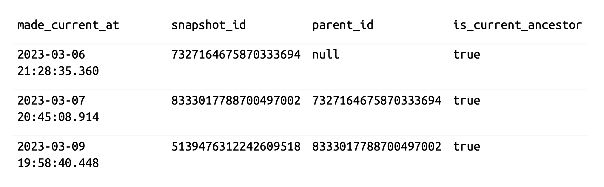
• e.g. to view the snapshot history, we can use the following query in spark -

  SELECT * FROM catalog.db.orders.history;
  

  

• running time travel queries using a timestamp -

  SELECT * FROM orders
  TIMESTAMP AS OF '2023-03-07 20:45:08.914'
  

• running time travel queries using a snapshot id -

  SELECT *
  FROM orders
  VERSION AS OF 8333017788700497002
  

Compaction

• the more files we have to scan for a query, the longer it will take
• this is because each file needs to opened, read and finally closed
• this problem is bigger in streaming queries, which creates a lot of files, each with a few records
• in contrast, batch ingestion plans all of this and writes the data as better, more organized files
• solution - rewrite all of the datafiles and manifests in smaller files into fewer, larger files

  Table table = catalog.loadTable("myTable");
  
  SparkActions
    .get()
    .rewriteDataFiles(table)
    .option("rewrite-job-order", "files-desc")
    .execute();
  

• compaction is smart enough to honor the latest partitioning spec - so, if the partitioning spec changes, the latest partitioning scheme would be used
• we should think of ways to run these maintenance jobs automatically on a schedule

Filter

• we can filter the files to rewrite by chaining the filter option
• e.g. below, we only rewrite the files of january

  .filter(
    Expressions.and(
      Expressions.greaterThanOrEqual("date", "2023-01-01"),
      Expressions.lessThanOrEqual("date", "2023-01-31")
    )
  )
  

• instead of using the java procedure, we can also use the rewrite_data_files procedure in spark sql

  CALL catalog.system.rewrite_data_files(
    table => 'musicians',
    strategy => 'binpack',
    where => 'genre = "rock"',
    options => map(
      'rewrite-job-order', 'bytes-asc',
      'target-file-size-bytes', '1073741824',
    )
  )
  

Options

this describes the various options we can add to the compaction process

• max-file-group-size-bytes - the workers (executors) will each write one file group. this helps with distributing the workload, concurrency, etc. e.g. if the memory of an executor is less than the total data in a partition, we can break a partition into file groups using this setting to ensure that each file group can be handled separately by an executor. max-concurrent-file-group-rewrites controls the max of number of file groups to write simultaneously
• partial-progress-enabled - commits can also happen during compaction. this helps read queries running in parallel to benefit from the compaction, if the compaction is long running. additionally, it also prevent oom like errors. when we enable partial progress, there would be multiple commits through the duration of the compaction. partial-progress-max-commits puts a cap on the maximum number of commits to allowed to complete the job
• recall - each parquet file is broken down into “row groups”. we can control the size of each parquet file and the size of row groups. more row groups in a parquet file = more metadata, more overhead but also more effective pruning / predicate pushdown. we can specify write.parquet.row-group-size-bytes and write.target.file-size-bytes at the table level settings. they default to 128mb and 512mb respectively. however, we can also specify them at the compaction job level, which uses the table level settings by default

Compaction Strategy 1 - Binpack

• it only combines files
• so, no global sorting
• effect - the data is not “clustered”
• advantage - quicker compaction jobs
• note - if there is a table level sort that has been defined, even if we do not specify the sort inside the compaction job, local sorting within each individual task will take place using this sort order specified in the table settings
• use case e.g. - meet slas in case of streaming workloads

  CALL catalog.system.rewrite_data_files(
    table => 'streamingtable',
    strategy => 'binpack',
    where => 'created_at between "2023-01-26 09:00:00" and "2023-01-26 09:59:59"',
    options => map(
      'rewrite-job-order','bytes-asc',
      'target-file-size-bytes','1073741824',
      'max-file-group-size-bytes','10737418240',
      'partial-progress-enabled', 'true'
    )
  )
  

• we need to balance out quick compaction jobs with performance. e.g. we can run one compaction job every hour for an hour of data, while one overnight for the entire day’s data

Compaction Strategy 2 - Sort

• sorting is also called “clustering”
• benefit - related data is collocated
• this reduces the number of files scanned. a lot of files can be removed from full scans during the query planning phase itself
• however, the faster reads come at the cost of more overhead in compaction jobs
• data is sorted by fields prior to allocating to tasks
• e.g. sort by a field a, then within that, sort by a field b
• we can specify the sort order property for a table as follows -

  ALTER TABLE catalog.nfl_teams WRITE ORDERED BY team;
  

Compaction Strategy 3 - ZOrder

• mostly same as sort
• however, fields are assigned equal weights in this case
• e.g. all values of field a within p-q are and field b within r-s are in one group and so on
• again, faster reads, at the cost of more overhead in compaction jobs
• rewrite files using zsort -

  CALL catalog.system.rewrite_data_files(
    table => 'people',
    strategy => 'sort',
    sort_order => 'zorder(age, height)'
  ) 
  

• even if we were filtering only by age, we would see performance improvements

Partitioning

• hidden partitioning - thus, we do not need to store data for additional columns
• queries of end users become intuitive. they can simply perform filtering etc using the original timestamp columns, instead of remembering to filter using an auxiliary column
• “year”, “month”, “day”, and “hour” transforms are allowed on a timestamp column to use for partitioning. e.g. if we use day, it will reflect the year, month and day of the timestamp
• we can also partition using the truncated value of a column, e.g. PARTITIONED BY truncate(name, 1) to partition using the first letter of name
• we can use the bucket transform for columns with lots of unique values i.e. “high cardinality”
• e.g. we want to filter using zip code - there can be lots of unique zip codes
• so, we can use the following - PARTITIONED BY bucket(24, zip)
• change the partitioning scheme midway - iceberg will track the two partitioning schemes separately
• it will instruct the engine to generate separate plans for both schemes

COW and MOR

• cow = “copy on write”, mor = “merge on read”
• read speed - copy on write > merge on read (position deletes) > merge on read (equality delete)
• write speed - merge on read (equality delete) > merge on read (position deletes) > copy on write
• we can set the approach at the table level, for the three operations - update, delete and merge

  ALTER TABLE catalog.people SET TBLPROPERTIES (
    'write.delete.mode'='merge-on-read',
    'write.update.mode'='copy-on-write',
    'write.merge.mode'='copy-on-write'
  );
  

• note - engines may or may not support mor, e.g. snowflake does not support mor currently

COW

• even if a single row is updated or deleted, the entire data file gets rewritten
• in copy on writes, reads are much faster, as no reconciliation is needed
• however, they are not ideal for use cases involving frequent row level updates

MOR

• working of updates -
  • add the record to be updated to a delete file
  • create a new datafile with just the new value of the updated record
• working of deletes -
  • add the record to be deleted to a delete file
• so, these need to be reconciled on reads
• note - for merge on read strategies, we should use frequent compactions for better read speeds
• use filtering strategies to run compactions on data that has been ingested in the last hour only
• also, use “partial progress” so that readers start seeing the benefits immediately
• there are two strategies for deletes - positional deletes and equality deletes
• “positional deletes” - will track which data file’s what record number needs to be deleted
  • advantage - fast reads
  • disadvantage - slower writes in comparison to equality deletes, since first a read operation is needed to identify the file and row number of the record to be deleted
• “equality deletes” - will just track the matching criteria for the records to be deleted
  • advantage - very fast writes
  • disadvantage - slower reads, since every record needs to be compared to check if they match the value in the delete files

Metrics Collection

• we saw how manifest files in iceberg for each of the columns track counts, null values, distinct values and upper / lower bound values
• if we have wide tables with a lot of columns, e.g. 100+, these metrics can become an overhead
• so, we can fine tune what metrics we want to track for what columns
• e.g. syntax of fine tuning this -

  ALTER TABLE catalog.db.students SET TBLPROPERTIES (
    'write.metadata.metrics.column.col1'='none',
    'write.metadata.metrics.column.col2'='full'
  )
  

• possible values -
  • “none” - do not collect any metrics
  • “counts” - track counts - values, distinct values, null values
  • “truncate(x)” - truncate(16) is the default. e.g. string values are truncated for calculating the metadata
  • “full” - track metadata based on the whole value

Rewrite Manifests

• sometimes, we have to read a lot of manifests
• we can consolidate all of the datafiles into a single manifest to speed up operations
• e.g. of running this -

  CALL catalog.system.rewrite_manifests('table')
  

• sometimes, we might run into oom issues due to spark’s caching. we can disable spark caching like so -

  CALL catalog.system.rewrite_manifests('table', false)
  

Optimizing Storage

• as we make updates or even run compactions - old files are not deleted, since they help with time travel
• we can periodically expire snapshots
• note - we cannot time travel back to expired snapshots
• example - it will expire all snapshots on or before the specified timestamp. however, it will not expire the snapshot if it falls within the last 100 snapshots

  CALL catalog.system.expire_snapshots('MyTable', TIMESTAMP '2023-02-01 00:00:00.000', 100)
  

• we can also instead specify the snapshot ids to expire etc
• another consideration to optimize storage is to delete the orphan files
• orphan files are files written by failed jobs, that never got cleaned

  CALL catalog.system.remove_orphan_files(table => 'MyTable')
  

• note - this operation is heavy, since it contains all kinds of metrics. so, it should only be run sporadically

Write Distribution Mode

• determines how mpp (massive parallel processing systems) handle writing data
• each task will write at least one file for each partition it has to write at least one record for
• assume we have 10 tasks and 10 records. assume they all belong to the same partition. if each record goes to a separate task, then each task creates a separate file. so, we end up with 10 different files, which is non ideal
• so, it would be better if all the records for a partition were allocated to the same task, so that lesser files are created
• modes -
  • none - no distribution happens. fast writes
  • hash - data is distributed based on hash of partition key. e.g. say we have values 1, 2, 3, 4, 5 and 6, while we have tasks a, b and c. values 1 and 4 go to task a, values 2 and 5 to task b and values 3 and 6 to task c
  • range - useful when we need to cluster data based on some attribute. e.g. values 1 and 2 go to task a, values 3 and 4 to task b and values 5 and 6 to task c
• we can also mix and match based on modes -

  ALTER TABLE catalog.MyTable SET TBLPROPERTIES (
    'write.distribution-mode' = 'hash',
    'write.delete.distribution-mode' = 'none',
    'write.update.distribution-mode' = 'range',
    'write.merge.distribution-mode' = 'hash',
  );
  

Object Storage Considerations

• recall how object storages work - there are limits on how many requests can go to a particular prefix
• one method to avoid such issues is compaction
• the other out of the box optimization inside iceberg is like so -

  alter table catalog.mytable set tblproperties (
    'write.object-storage.enabled'= true
  );
  

• so, instead of this -

  s3://bucket/database/table/field=value1/datafile1.parquet
  s3://bucket/database/table/field=value1/datafile2.parquet
  s3://bucket/database/table/field=value1/datafile3.parquet
  

  we will get this -

  s3://bucket/4809098/database/table/field=value1/datafile1.parquet
  s3://bucket/5840329/database/table/field=value1/datafile2.parquet
  s3://bucket/2342344/database/table/field=value1/datafile3.parquet
  

Bloom Filters

• how bloom filters work
  • say we have records, which we can represent using 5 bits
  • now, say one of the records is represented as 10001
  • then, we run it through a hash function
  • say it returns the 5th bit
  • since 5th bit is 1 - we mark the 5th bit in the bloom filter as 1 as well
  • what this means - if a record hashes to 5th bit, it “could be” present in the dataset, since the bloom filter is marked 1 for it
  • say a record hashes to 4th bit. since the bloom filter holds 0 for the 4th bit, we can be sure that the value “would not” be present in the dataset
• we can enable bloom filters for certain columns, and configure its size
• however, the bigger it gets, the more overhead it incurs
• example -

  ALTER TABLE catalog.MyTable SET TBLPROPERTIES (
    'write.parquet.bloom-filter-enabled.column.col1'= true,
    'write.parquet.bloom-filter-max-bytes'= 1048576
  );
  

Catalog

• iceberg catalog is an interface, that exposes multiple functions to create, rename, drop tables etc
• there are multiple implementations of it like glue, hive, etc
• primary requirement - map the table name in catalog to the metadata file representing the current state
• example of how it is handled by different catalogs -
  • file system catalogs like hadoop - store a file called version-hint.txt that points to the right metadata file
  • hive metastore - table has a property called location to point to the right metadata file
  • glue uses a similar approach - track using metadata_location
• cons of glue -
  • does not support multi table transactions
  • specific to aws - not for multi cloud solutions
• nessie -
  • works like git - versioned like source code. this helps with safe changes, reproducibility, traceability, etc
  • supports multi table / multi statement transactions
  • we host the infrastructure ourselves, while dremio etc also offer managed workflows

Spark

• we can also use SparkSessionCatalog instead of SparkCatalog. advantage - helps us use iceberg tables seamlessly alongside non-iceberg tables. non-iceberg tables are managed by the built-in spark catalog
• we can either use specify packages like here, or add the jars to the artifact and specify that path using --jars
• in the below example, glue after spark.sql.catalog is the “catalog name”. it can be anything
• with the iceberg extensions module, we can execute statements not part of standard sql - like calling maintenance procedures
• full example for glue. remember to set the environment variables AWS_REGION, AWS_ACCESS_KEY_ID and AWS_SECRET_ACCESS_KEY -

  import pyspark
  from pyspark.sql import SparkSession
  import os
  
  packages = [
    'org.apache.iceberg:iceberg-spark-runtime-3.3_2.12:1.2.0',
    'software.amazon.awssdk:bundle:2.17.178',
    'software.amazon.awssdk:url-connection-client:2.17.178'
  ]
  
  conf = (
    pyspark.SparkConf()
      .setAppName('app_name')
      .set('spark.jars.packages', ','.join(packages))
      .set('spark.sql.extensions', 'org.apache.iceberg.spark.extensions.IcebergSparkSessionExtensions')
      .set('spark.sql.catalog.glue', 'org.apache.iceberg.spark.SparkCatalog')
      .set('spark.sql.catalog.glue.catalog-impl', 'org.apache.iceberg.aws.glue.GlueCatalog')
      .set('spark.sql.catalog.glue.warehouse', 's3://my-bucket/warehouse/')
      .set('spark.sql.catalog.glue.io-impl', 'org.apache.iceberg.aws.s3.S3FileIO')
  )
  
  spark = SparkSession.builder.config(conf=conf).getOrCreate()
  

• we can use the dataframe api or sql. dataframe api might have limitations
• notice how glue below is the catalog name (refer above) and we tell spark to use the iceberg table format

  create table glue.test.employee (
    id int,
    department string,
    join_date date
  )
  using iceberg
  partitioned by months(join_date);
  

• alter table contrived examples -
  • setting table properties - alter table glue.test.employee rename to glue.test.employee_renamed
  • wap is write-audit-publish. it is a method to stage writes before publishing them. alter table glue.test.employee set tblproperties ('write.wap.enabled'='true')
  • use first / after clauses to change positions of columns - alter table glue.test.employee alter column salary after department
  • add a partition field - alter table glue.test.employee add partition department
• window functions - they do not group rows into a single output like aggregations. instead, they perform calculations across a set of rows for the current row. e.g. rolling average, rank items, etc

  select *, rank() over (
    partition by department
    order by salary desc
  ) as rank
  from glue.test.employee
  

• merge into - if the condition is matched, the row is updated. if not, the new row gets inserted into the table. also, notice how we can add additional conditions to the when matched clause as well

  merge into glue.test.employee as target
  using (select * from employee_updates) as source
  on target.id = source.id
  when matched and source.role = 'manager' and source.salary > 100000 then
  update set target.salary = source.salary
  when not matched then
  insert *
  

• insert overwrite - used to replace the data in an iceberg table / partition with the result of a query
• it is of two types - static and dynamic
• static - iceberg determines the partitions to overwrite using what we specify in the partition clause. note - this will not work for dynamic partitions, since the partition clause can only reference table columns

  insert overwrite glue.test.employees
  partition (region = 'emea')
  select *
  from employee_source
  where region = 'emea'
  

• dynamic - any partition that matches the data returned by the query gets replaced. for this, we first need to set spark.sql.sources.partitionOverwriteMode to dynamic
• delete from - iceberg can perform two kinds of deletes. if the filter condition matches entire partitions of the table, only the metadata files are updated, and the datafiles are untouched. so, this kind of delete is very optimal. otherwise, iceberg will write the affected files

  delete from glue.test.employee where id < 3
  

• updating based on a subquery -

  update glue.test.employee as e
  set region = 'na'
  where exists (select id from emp_history where emp_na.id = e.id)