Data Engineering

Different Architectures

• oltp -
  • online transactional processing
  • used for operational data keeping
  • we do not maintain a history of the data - we update records in place to reflect the current state of the system
• olap -
  • online analytical processing
  • used for analytical decision making
  • it contains historical data as well, not just the current data
  • millions of records are analyzed at a time, so we need fast query processing
• data warehouse -
  • “centralized location” for all external otlp data sources - we basically copy the data from these different sources into a single place
  • two reasons for using data warehouses -
    • “optimized” for analytic processing
    • should also be “user friendly” for decision makers
  • must load data consistently and repeatedly using “etl”
  • note - ensuring “non volatility” is important during etl - our data warehouse should be consistent between the etl refreshes that we do on a scheduled basis - warehouse can go into an inconsistent state “during” an etl refresh, ensure that does not happen
• data lake -
  • was needed to accommodate for three vs - volume, velocity, variety
  • because of this, technology used by data lake is big data, while warehouses use databases
  • used when the use case is not properly defined yet
  • used for storing raw data. data is not stored in processed format like in warehouse
  • so, modern day data lake architecture looks like this -
    • get data in raw format from source systems into lake using systems like kafka etc
    • the lake storage can be hdfs, s3, azure blob storage, etc
    • perform some processing using technologies like spark
    • finally, write to systems like relational databases to support use cases like reporting
• data virtualization -
  • in data warehousing, we duplicate the data and transform it to optimize it
  • in data virtualization, we access it from its original source itself
  • we access data from different sources “in the same way”, agnostic of the underlying database
  • so, this technique is useful when we are okay with the larger response times, require minimum transformations on the raw data, etc
• etl -
  • extract, transform, load
  • “extract” - bring the raw data as is into the staging layer
  • “transform” - perform transformations to create a dimensional model of the data
  • “load” - load into the core / user access / warehouse layer
  • it is typically done in batches
• ods -
  • operational data storage
  • used for “operational decision making” and not analytical decision making
  • there is a need for “realtime” unlike in data warehouses, where we do batch processing
  • the architecture we are talking about here is that from the actual sources, we have two separate things spawning off - the ods and the the actual warehouse
  • another architecture - we can treat ods as the staging layer of the warehouse, and then perform batch “tl” on this staging layer for constructing the warehouse layer
• elt -
  • problem with etl - a lot of data modelling and understanding of business use case is needed before storing the actual data
  • instead, we flip the order of transform and load
  • we “blast” the data into a “big data environment” in their raw form
  • then, we use the compute of the warehouse / big data to perform transformations
  • elt allows for much more flexible transformations as compared to etl, since in etl, we perform transformations to load data into the core layer, while the transformations move towards the client in elt
  • with traditional data warehouses, we still use etl, but when we use the newer paradigms like data lakes etc, we start utilizing elt patterns
• we can build on prem or cloud, both have their own considerations. e.g. egress data from cloud is usually much more expensive than ingress data into cloud

Technologies in Warehouses

• relational databases - uses popular sql for querying, primary keys and foreign keys, etc - relational databases are also a great starting point for storing our warehouses
• cubes -
  • data is stored in a multidimensional array
  • e.g. imagine we want sales for a particular customer and product, the value will already be aggregated across remaining dimensions like time
  • it uses the mdx language for querying
  • so, optimizations like pre computations, indexing, etc underneath make cubes very fast for complex queries
  • extra “cost of compute” to maintain these complex structures
  • so, imagine the recomputation in aggregations needed in case of updates
  • earlier, cubes were an alternative to dimensional modelling and building warehouses using technologies like rdbms
  • now, cubes can be seen as a specialized technology for the data mart layer
• in memory databases - for high query performance, used in for e.g. data marts. in traditional databases, data is stored in hdd / ssd in disk and loaded into memory for querying. this is eliminated here to increase performance. challenge - lack of durability, resolve via snapshots / images to help restore to a specific point. e.g. sap hana, amazon memory db, etc
• columnar storage - traditionally, queries are processed row wise. if we use columnar storage, data is stored column wise. so, if we need to process only a small subset of columns, we do not have to process entire rows and go through all the data like in traditional relational databases
• massive parallel processing - a task can be broken down into multiple subtasks. this way, these subtasks can run in parallel, thus optimizing performance
• in mpp above, we talked about breaking down compute. for scaling storage, the underlying architecture can be -
  • shared disk architecture - underlying storage is one i.e. multiple computes run on top of the same underlying storage
  • shared nothing architecture - underlying storage is also broken down i.e. each compute will have its own storage

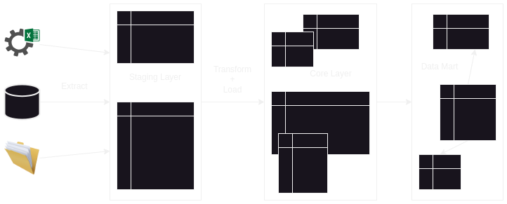
Warehouse Architecture

• we put the data “as is” into the staging layer of the warehouse
• we can do some minute transformations like renaming and adjusting positions of columns when performing a union between employee datasets from different sources
• we put the data into the core / user access / warehouse layer by performing transformations from the staging layer
• why do we need a staging layer i.e. why not load into the warehouse layers directly from the sources -
  • we risk burdening our oltp systems
  • also, data from sources can be in different formats like crm, files like xml, etc. we get all the data from these different sources into for e.g. a relational db, which helps us use sql / a standard way to perform transformations, e.g. perform joins easily which would not be possible otherwise when data comes from different sources
• staging layer can be temporary (more common) or permanent
• temporary - after the data is loaded into the warehouse layer, we truncate the staging layer. this way, the next time we want to load data into the warehouse layer, we need to perform a diff - we need to know the last inserted row inside the warehouse layer, and calculate the new rows inside the sources since then, and accordingly add the new data to the warehouse. this diff checking can be done on columns like timestamp if maintained
• persistent staging layer - maybe easier since existing warehouse layer can be recreated / new warehouse layers can be created easily
• we can either consume from the core layer directly, or have data marts on top. some use cases of having data marts -
  • core layer has a lot of tables - we can have data marts on top of this. now, users will only have access to tables which they need
  • core layer isn’t burdened with queries from all consumers, and consumers only consume capacity of their data marts
  • allow us to have different types of databases, e.g. in memory vs cubes based on use case
  • other concerns like security are separated as well
• on a higher level, there are two options - “centralized” and “component based”
• “centralized” - one warehouse layer, and consumers consume from this layer. advantage - “one stop shopping” for all our consumers. here, we have two options -
  • “edw” (enterprise data warehouses) - typical relational databases, columnar storages, etc
  • “data lake” - big data technologies like hadoop, s3, etc
• “component based” - each consumer has its own data mart. advantage - allows for mix and match of technology based on use case. here, we have two options -
  • “dependent data marts” - this is the variation we have seen - data marts are built on top of the warehouse layer
  • “independent data marts” - in this, we skip the warehouse layer. we make data marts directly consume from the sources and perform transformations. so, it is like we have small warehouse layers per consumer
• general rule - we should strive towards “centralized” instead of “component based”
• initial load -
  • first extraction
  • it is much slower and puts load on sources, so it is best if done during weekends etc. so that the systems are not impacted
  • we can use it for fault tolerance later on as well, in case the warehouse ever gets corrupted
  • note - we are talking about a warehouse. this does not include only data of “current state”, but “historical data” as well. recall that typically, only the current state of the system stored in the otlp databases, so we might need to support the audit trail of data somehow
• delta / incremental load -
  • incrementally loading (new / modified / deleted) data
  • uses fields like timestamp (created / modified date) etc
  • note - for processing deletes, we use delete markers instead of actually deleting the data
  • we run it on a schedule regularly instead of just once
  • we also run it on a subset of data by filtering out and retaining only the new / modified data
• incremental load patterns -
  • “append” - append new information
  • “in place updates” - we make changes to existing data when applying updates
  • “complete replacement” - we overwrite the entire data completely, even if only a small subset of it changes
  • “rolling append” - say we only maintain a window of lets say 2 years of data. so, when we receive a sales event, we expire all the data that is more than 2 years before it

• typically, we use append for fact tables, and in place updates for scd 1 / append for scd 2. so, the incremental load patterns’ decision is scoped to a “table”, not an entire dimensional model

  

• transformation examples -
  • deduplication - e.g. two campuses somehow have duplicate information about the same faculty, because this faculty takes classes in both campuses. we might want to deduplicate this faculty information when creating our dimensional models
  • filtering out rows / columns
  • data value unification - e.g. when performing a union, one source system contains m and f, while another contains male / female
  • key generation - surrogate key
  • joining
  • splitting - e.g. if natural keys are composed of the division and department codes, split them into individual columns
  • aggregations / groupings
  • deriving columns - precalculate profit using sales, costs, discounts

Dimensional Modelling

• “dimensional modelling” - it is a method of organizing data, which helps with two major concerns
  • “usability” - business users should be able to understand it easily - several instances have shown how business users immediately understand this
  • “performance” - querying it should be very fast. this method of organizing data helps with optimizations underneath, e.g. our queries would typically first filter out the rows in the dimension tables, and then perform joins with the fact table
• note - dimensions modelling is organizing tables into facts and dimensions. but, based on use case, we can also rather organize data as flat tables in our warehouse, e.g. join and group data to produce the final aggregated form directly, instead of expecting our end users to perform aggregations
• facts - represent a single measurement, e.g. an order line
• dimensions - “give context” to the measurements e.g. product category
• important - dimensions help in “grouping” / “filtering” facts for our use case. grouping and filtering is key here - we need to be able to derive this ourselves
• e.g. if our fact is student loan, and we want to derive insights “for” engineering major “by” department, we need to use where clause for major and group by department
• identifying facts -
  • are measurable - we can perform some calculations on them
  • facts can also mark events sometimes, which is why it is accompanied by a date
• grain - the most atomic level of a fact table - what does a row in the fact table actually represent. keep it fine level for flexibility, this way we can do aggregations for summaries
• we usually have multiple dimensions clustered around the fact, thus it is called a star schema - the structure looks like that of a star, with the fact table at the center and the dimension tables at the tips of the star spiking out of the fact table
• dimension tables have more attributes / are much wider when compared to fact tables
• however, fact tables have much more records than dimension tables
• maybe thats why we use delta load for fact tables and full load in dimension tables sometimes
• indexes - make reads faster, writes slower. useful when we join, filter by, etc. on the data based on that column
• b tree index - this is the default / most common type of index. we can break data into a multi level tree. helpful when column has high cardinality
  

• bitmap index - useful when the column has a low cardinality. the position of bit corresponds to the row number, and if its 1, it means that row has that value

  pk	payment type
  1	visa
  2	mastercard
  3	mastercard
  4	visa

  payment type	bitmap
  visa	1001
  mastercard	0110

• fact table indexing example - using b tree index on surrogate key and bitmap index on the dimension column foreign keys
• tips for fact tables -
  • avoid bloating the fact table for increased performance. even if it is one to one, move the contextual data into a separate dimension table
  • my understanding - i think the above point is even more important, considering facts are never updated, only dimensions are updated using slowly changing dimensions. so, we cannot store context in fact tables, since it cannot be updated
• tips for dimension tables -
  • try replacing cryptic abbreviations with real words to decrease reliance on lookups etc
  • sometimes, ids have a special embedded meaning, e.g. first three letters represent the department. extract these into separate columns beforehand instead of having business users query on these attributes
  • denormalization or data redundancy might be used in dimension tables to help with query performance, e.g. the column category in the product dimension table discussed above, notice the repeating category snacks. data warehouses are not maintained using 3nf models, if we do so, we are creating a snowflake schema
  • index dimension tables properly - since operations like filtering etc are performed on dimension tables, we should index them properly
• snowflake schema -
  • a star schema is a snowflake schema with one level
  • e.g. the product dimension table will be a join between the product and category tables, thus making it denormalized
  • if the denormalization above is actually degrading our performance / affecting our consistency, we can instead have multiple levels e.g. the category column can be extracted into its own dimension table in the product dimension table
  • so, when we have multiple levels of dimension tables like this, it is also called a snowflake schema
  • note it can result in multiple joins, thus degrading performance, but consume lesser storage at the same time
• surrogate keys -
  • use auto generated integer ids / a key management service instead of natural keys
  • they are more performant compared to natural keys which are usually strings
  • we can also use -1 for dummy dimensions discussed below to make our intent clearer
  • we can still retain the natural keys, but the warehouse and its users use the surrogate keys to perform joins etc
• exception to above - date dimensions - foreign key / surrogate key in date dimension does not have to be meaningless auto incremented integers. instead of an auto incremented integer, represent the actual date time as an integer, e.g. 050820232232 (first 8 characters represent date, remaining 4 time)
• so, the final architecture (in terms of keys) looks like this -
  • dimension tables have surrogate keys as their primary key
  • however, the dimension tables can still retain the natural key columns
  • the fact tables use the composite key comprising of all the foreign surrogate keys as their primary key
  • however, the fact tables can still retain the natural key columns
• it is common to keep pre calculated aggregates in the fact table, e.g. instead of expecting users to perform addition / subtraction to get the profit earned per order line item, just maintain it as a separate column in the fact table which can be used. this way users do not perform erroneous calculations
• date dimension - pre calculated values like day of week, month name, etc. since date dimension is very predictable, we can pre-populate the date dimension table for the next 10 years or so in advance. we can also consider populating all variations, e.g. month full name, month abbreviation, month as integer in case of date dimension

Additivity in Facts

• note - additivity includes adding only, not average etc

• “additive facts” - can be added across all dimensions. e.g. adding units sold across the date dimension tells us the number of units sold for a particular product, adding the units sold across the product dimension tells us the number of units sold at a particular date. note - i get confused in terminology. across product means group by date

  product_id	units sold	date	price
  1	2	06082023	23
  2	2	06082023	19
  1	5	10082023	11

• “semi-additive facts” - only added across some dimensions. e.g. imagine a fact table where the grain is our balance on a particular date for a particular folio

  portfolio_id	date	balance
  1	06082023	100
  2	06082023	50
  1	10082023	110

• adding balance across the date dimension does not make sense, since balance is a cumulative number

  portfolio_id	balance
  1	210
  2	50

• but adding it across portfolios tells us our total balance on a particular date

  date	balance
  06082023	150
  10082023	110

• “non-additive facts” - cannot be added across any dimension. e.g. price of a product. if products make up our fact table, there is no meaning of summing the prices of different products
• nulls for facts in fact tables - usually in tools, average ignores null, sums will treat nulls as a 0, etc. but sometimes, we might want to replace nulls with 0, it depends on our use case
• nulls for foreign keys in fact tables - nulls can result in problems, therefore introduce a row in the dimension table with a dummy value, and have the rows with null as foreign key in the fact table point to this dummy value’s primary key instead

Types of Fact Tables

Transactional Fact Table

• a grain indicates one event / transaction
• e.g. one row represents one meal payment -
  • dimensions are date, the counter and the student
  • the fact is the actual amount
• the fact table will look as follows (recall how primary key of a fact table is a composite key constructed using the surrogate foreign keys for dimension tables) -
  • student_id (pk, fk)
  • counter_id (pk, fk)
  • date_id (pk, fk)
  • amount (double)
• characteristic - will have “many dimensions” (foreign keys)
• disadvantage - “grow very rapidly” in size, and queries on such facts often require aggregations
• we can store two or more facts in this fact table, if the “two rules” below are met -
  • facts occur at the same grain
  • facts occur simultaneously
• e.g. tuition bill and tuition payment -
  • they occur at the same grain - both have similar dimensions - student, date, etc
  • but, they occur at different times, since they are different business processes
  • so, they cannot be stored in the same transactional fact table
• e.g. tuition bill, hostel bill and co curricular activities bill -
  • they can be stored in the same fact table as they satisfy both rules
  • so, the fact table will have 3 different facts for the 3 amounts
• assume tuition and co curricular activities had a campus component in them, which the hostel did not
  • facts do not occur at the same grain - hostel does not have the same dimensions as the other two
  • so, we cannot store the three facts in the same fact table

Periodic Snapshot Fact Table

• a grain is a “summary of transactions”
• sometimes, it is possible to do this using the transaction fact table, but for e.g. the sql can get complex
• so, we can instead answer specific business questions using periodic snapshot fact tables
• e.g. analyze end of week balances for a customer. fact table -
  • student_id (pk, fk)
  • week_id (pk, fk)
  • balance
• characteristic - because of its nature, it “will not have many dimensions”, since a row is an aggregation across some dimension(s)
• advantage - they “grow slower” compared to the transactional fact table
• typically, they are “semi additive” - because the fact here is a summarized value, we cannot add it across all dimensions as easily as a transactional fact

Accumulation Snapshot Fact Table

• one grain summarizes the “progress of a business process” defined through different stages
• e.g. one row represents an order, which has stages for production, packaging, shipping, delivery, etc
• characteristic - it “has many date dimensions”
• so, date is also an example of “a role playing dimension” for us
• this too should grow slower in size as compared to the transactional fact table

Factless Fact Table

• sometimes, there is no measurable fact
• e.g. a fact table where a new record for every new employee that is registered
• it will have dimensions like department id, employee id, position id, date, etc, but no measurable fact
• we can perform aggregations to answer questions like -
  • number of employees who joined last month
  • number of employees in a department
• another technique - “tracking fact”
  • we store a boolean value - can be set to 1 or 0
  • e.g. the fact table represents a student “registering” for a webinar
  • but, we store 1 or 0 depending on whether or not the student actually attends the webinar
  • now, we can perform sum aggregation to get the number of students who actually attend the webinar

Types of Dimensions

• “conformed dimensions” - dimensions shared across multiple facts, e.g. date dimension. advantages -
  • helps combine the facts using the shared dimension. e.g. if we have two different facts for sales and profits, we can combine them using the date dimension. this helps us compare the cost and sales side by side
  • we can reuse the same dimension table across different dimensional models - this way, we save on the etl / storage costs of maintaining duplicate dimension tables
• “degenerate dimension” - e.g. we have a sales fact table, with a foreign (surrogate) key for the category dimension. the category dimension only has two columns - the surrogate key and the category name. so, we can instead directly store the category name in the sales fact table. this usually occurs in the transactional fact table
• “junk dimensions” - e.g. imagine we have a lot of indicators that are eating up a lot of width (therefore space) of the fact table, thus impacting its performance. so, we can instead extract these dimensions to its own table. note - the “cardinality” of these dimensions should be “low”
• typically, we store all the possible values in the junk dimension. but, the number of rows in this junk dimension can grow a lot, e.g. m, n, p, q values for 4 columns respectively will mean a total of m * n * p * q combinations. so, we can -
  • store the dimensions “as we come across them” in this junk dimension instead of storing all combinations in a precomputed fashion
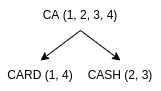
  • “split” the junk dimensions i.e. group related junk dimensions together. advantage - now, one junk dimension table will have m * n values, another will have p * q values

  amount	payment_method	incoming / outgoing
  23	credit card	incoming
  12	cash	outgoing

  amount	flag
  23	1
  12	3

  pk	payment_method	incoming / outgoing
  1	credit card	incoming
  3	cash	outgoing

• “role playing dimension” -
  • same dimension table is referenced in the fact table multiple times
  • e.g. date dimension for order date vs shipping date. note - this is also an example of accumulation snapshot fact table
  • an additional optimization for bi - use views - data is not duplicated, but users see different dimension tables for the different “roles” the date dimension might be playing, thus increasing readability

Slowly Changing Dimensions

• we have different techniques to manage changes in dimensions
• my realization - data in fact tables is never updated, it has insert only operations. this means it makes even more sense to move out data that is not “measurement related” from the fact table

Type 0

• only retain the original data
• useful when our dimensions do not change. e.g. date dimension

Type 1

• we overwrite the old data in the same row with the new values for its columns
• so, no history is retained
• e.g. a new category for biscuits was introduced. so, the category changes from snacks to biscuits
• issue - this can suddenly kind of maybe show reduced sales for dashboards which were monitoring the category for snacks

Type 2

• add new rows for the new versions, instead of updating existing rows as in type 1
• so basically, now we have a new row with a new primary surrogate key in our dimension table
• disadvantage - most complex to implement
• advantage - most accurate representation of history

• e.g. old financial aids will point to the older student dimension row, and newer financial aid will point to the newer student dimension row

  financial_aid_key	student_key	amount
  1	2	500
  1	3	200
  1	4	750

  key	name	level
  2	john doe	higher secondary
  3	michael smith	higher secondary
  4	john doe	college

• issue 1 - how can we get all financial aids for a student? my understanding - we will have to use the natural key stored in the dimension table, student_id in this case. e.g. we can fetch all the keys corresponding to the student_id for which we need the financial aids, then we can join it with the fact table for all the financial aids for this student

  key	name	level	student_id
  2	john doe	higher secondary	87555
  3	michael smith	higher secondary	54568
  4	john doe	college	87555

• issue 2 - we do not have a way of telling for e.g. the current categories in our system, since we now have multiple rows
  • option 1 - we can have a boolean attribute is obsolete, which will be marked 1 for all the newer versions, and 0 for all the older versions. issue - we cannot predict the “order of updates”, in case there are 4-5 updates for the same student
  • option 2 - introduce an effective and an expiry date. it helps maintain the ordering as well
  • option 3 - use both. this is the recommended approach by kimball

  key	name	level	student_id	effective_date	expiry_date	is_active
  2	john doe	higher secondary	87555	06082023	08082023	0
  3	michael smith	higher secondary	54568	06082023	31129999	1
  4	john doe	college	87555	08082023	31129999	1

Type 3

• we introduce a new columns for the different versions, as opposed to inserting new rows as in type 2
• advantage - allows to switch back and forth between different versions easily
• so we will have two columns - previous category and current category in the category dimension table
• it is not for unpredictable / frequent changes, we use type 2 for that
• this is for a more structured change like a reorganization at a company
• this way, we can lay out a clear demise plan in place with maintaining backwards compatibility

ETL Design

• our etl design is guided by our decisions of -
  • type of slowly changing dimensions we use
  • how we do cdc (change data capture) i.e. recall the kind of incremental loads we can use
  • type of fact table in our dimensional model
• there are different ways to do cdc -
  • we can use the timestamp of the transaction. we can use the “watermark” for this - we keep track of the last etl run’s timestamp. based on the value of the watermark, we need to look for new / updated data in the sources
  • we can also use the “database logs” directly - debezium i believe uses this
• we should also have some kind of “parallel processing” for more efficiency. however, we have to process dimension table changes before processing the fact table changes. even the dimension table changes need to be processed in order of dependency if we have a snowflake schema instead of a star schema
• for dimension tables -
  • new data - we can look for natural keys in the source not present in our dimension table. then, we can insert them by additionally adding a surrogate key to them
  • type 1 change example - “update all rows”. why all rows - if a type 2 change for a different column occurs before the type 1 change for this column, we will have to update all the rows with the same natural key with the new value. why - when analyzing, it might happen that the older version of the dimension is relevant - we would still want the latest value for this column in the older version
  • type 2 change example - we add a new surrogate key. the natural key stays the same however. we can update the effective / expiry date columns accordingly as well
• for fact tables -
  • we need to get “the right row” from the dimension table, because there can be multiple rows for the same natural key due to type 2 scd. after this, we can add the new fact, if present, using the surrogate key of this latest dimension