Interview Pointers
- clear both functional and non functional requirements
- questions about data
- what is the current size of data?
- what is the rate of incoming data?
- what is the durability requirement for the data?
- is the system read heavy or write heavy?
- what consistency guarantees do we need for our data?
- “back of the envelope calculations”
- how many concurrent users use our system at a time?
- how many requests per second reach the server, cache, etc
- reference - while this would greatly differ based on the kind of system, these are some approximate numbers -
- mysql - 1k qps
- key value store - 10k qps
- cache server - 100k qps - 1mil qps
- while doing the above, remember that requests can be of different types -
- cpu bound - compression of data
- memory bound - reading from ram
- io bound - reading from disk, network
- discuss the components - load balancers, types of databases and caches, etc
- my thought - try applying and discussing all possible patterns we learned, e.g. saga, cqrs, etc
- point of the trade offs we make - e.g. concurrency control (pessimistic vs optimistic) and so on
Request Estimation Calculation
- how many requests a server can handle -
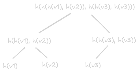
- time per program = instruction per program * clock cycles per instruction * time per clock cycle
- assume each instruction takes 1 clock cycle
- assume average clock rate is 3.5ghz. so, 3.5 * 10^9
- a request is typically a few million. assume 3.5 million for simplifying calculation
- so, time per program = (3.5 * 10^6 * 1 * (1 / (3.5 * 10^9)))
- so, 1 request takes 1 millisecond of a cpu core
- so, in second, 1 core can handle 1000 requests
- so, a typical 64 core cpu can handle 64k requests
- now, assume we have 500 million users, and each of them make 20 requests a day on average
- that is 115 requests per second, or we need 2 servers to handle it (recall 64k earlier)
- of course, we are making assumptions, e.g. requests are spread uniformly. e.g. 20 requests a day need not be evenly spread out. this means we will need more cpus to handle a higher load
- storage handling (example twitter) -
- handle image size (e.g. 100kb), video size (e.g. 1mb), and content (e.g. 250 bytes) separately
- also, factor in that for e.g. only 20% tweets will have images, and only 5% will have videos
Load Balancers
Types of Load Balancers
- “stateful” vs “stateless” -
- stateful load balancers would maintain the state between client and server
- since there would be multiple load balancers, they need to coordinate this state with one another
- hence there is maintenance overhead, since session information for all the clients needs to be maintained across all the different load balancers
- if we use stateless load balancers, it would use consistent hashing to route to the right server
- issue - if for e.g. we add a new server, the request from the same user would now go to a different server. hash(user_id) % 3 and hash(user_id) % 4 have different results
- solution - the stateless load balancer maintains a local state to help with this
- so, “stateful load balancers” maintain a global state synchronized across all load balancers, while “stateless load balancers” might only maintain local state
- “layer 4” vs “layer 7” -
- “layer 4” - load balancing is performed using tcp / udp
- “layer 7” - based on application layer protocols
- layer 4 can support forwarding of same tcp / udp communication to the same backend server, tls termination, etc
- layer 7 however supports “application aware” load balancing i.e. based on url, cookie, etc
- this “inspection” makes it relatively slower than layer 4 load balancers
Load Balancer Deployment
- “tier 1 load balancer” - simply route the request to tier 2 load balancer
- they use ecmp “equal cost multi path” routing i.e. request can be routed through various paths with the same priority (maybe because they result in similar performance)
- so, it is like tier 1 load balancer can route to any tier 2 load balancer
- “tier 2 load balancer” - glue between tier 1 and tier 3 load balancer
- they can be stateful or stateless
- however, they ensure that the request gets routed to the same tier 3 load balancer every time
- they use layer 4 load balancing
- “tier 3 load balancer” - this is where the actual load balancing happens, i.e. the request gets routed to the appropriate backend service
- also, it handles load balancing between the different servers of the particular backend service
- they use layer 7 load balancing
- they do things like performing health checks on the servers, tls termination, etc
Databases
Data Replication
- store multiple copies of data at various nodes - preferably geographically distributed
- this helps with both reliability and performance
- important - if asked to increase read performance, think replication instead of sharding
- “synchronous replication” - primary node first writes to itself, then waits for acknowledgement from the secondary nodes to complete the write as well
- “asynchronous replication” - primary node does not wait for acknowledgement from the secondary nodes
- “single leader / primary secondary replication” -
- one node is designated as primary
- it keeps the follower replicas in sync
- good for read intensive applications
- bad for write intensive applications
- inconsistency if asynchronous replication is used
- in case the primary node fails, one of the secondary nodes can be promoted to primary
- “multi leader replication” -
- single leader has performance concerns - the single primary node can become a bottleneck
- tools like “tungsten replicator” for mysql can be used
- e.g. when we are offline, we can continue working and when we come back online, our changes are synced to the servers. in this case, our device is like a primary node as well
- issue - “conflicts” - multiple writers overwrite the same row from different replicas at the same time. e.g. primary node 1 gets x and primary node 2 gets y. then, node 1 tells node 2 to write x, while node 2 communicates to node 1 to write y
- solution 1 - “last write wins” - the replicas also assign a timestamp to each write
- solution 2 - “custom logic” - we have our own custom logic, that can be either executed at the write time, or for e.g. deferred to during the read
- “peer to peer / leaderless replication” -
- all nodes have equal weights, and can accept both reads and writes
- this can have even higher chances of inconsistency
- solution - “quorum”
- writes should reach at least w nodes for it to be a success, and we should read from at least r nodes
- we will get updated values as long as w + r > n
- now, we discuss replication methods
- “statement based replication” -
- the statement is executed on the primary node
- this statement is captured in a log file
- then, this log file gets sent to other nodes
- disadvantage - non deterministic functions like
now()might have different values
- “write ahead log replication” -
- like sbr, but instead wal (write ahead log) files are used
- wal files capture the transactional logs instead of statements
- disadvantage - tightly coupled with db engine, making software upgrades on leaders and followers tough
- “logical replication / row-based replication -
- changes made are captured at the level of individual rows
- then, these changes are replicated
- e.g. in case of an update, the entire row is captured and then executed on the other nodes
Data Partitioning
- relational databases have scalability challenges
- however, they are attractive due to their benefits - “range queries”, “secondary indices”, “transactions”, etc
- we can use nosql databases, but there is effort around migration etc
- so, with “sharding” / “partitioning”, each node only handles some part of the data
- “vertical sharding” - putting different columns of a table / tables of a database in different shards
- e.g. put all columns of employee table in one shard, and its blob columns like picture in another
- one shard has the table (id, name) and another shard has the table (id, picture)
- “horizontal scaling” - we split the data row wise. it has 2 strategies - “key range based” and “hash based”
- “key range based sharding” - each shard is assigned a continuous range of keys
- when we have multiple tables in a database bound by a foreign key. we use the same “partition key” throughout for all the different tables in this case
- for performance etc, we should try keeping tables appearing in joins in same shards
- e.g. if we say customers with ids 1-10 belong to shard 1, then all their invoices, invoice line items, etc should have the customer id column and also belong to the same shard
- slight trade off - increased storage due to the extra customer id column, not normalized anymore, etc
- “key range based sharding advantage” - we can easily perform range based queries. we can also keep them sorted by the partition key for even faster performance
- “hash based sharding” - same as key range based sharding, but we use hash(key) % no. of shards instead of the partition key to determine the shard
- advantage - fewer chances of “hot partitions” / “data skew”
- disadvantage - cannot perform range queries anymore
- “consistent hashing” - this means servers and items get a place in an abstract circle
- advantage - allows both the servers and items to scale horizontally easily
- calculation example - assume we would like to have 100tb of data and 50gb per shard
- this means we would need 200 shards in total
- “rebalancing” might be needed to avoid hot partitions, to handle increase in overall traffic, etc
- e.g. in “dynamic partitioning”, once a partition reaches a threshold, split it into two partitions. disadvantage - performing this rebalancing dynamically is difficult, when we are also performing reads and writes simultaneously
- now, what if we wanted to retrieve documents using “secondary” instead of “primary” index? assume customer name is our secondary index. we can use one of the two techniques below -
- “partition secondary indices by document” - each shard has its own secondary index. this is also “local secondary index”. the partitions are not concerned with each other. so, lets say for e.g. we want to search for customers with the name john. we will request all the shards for this name. disadvantage - increased read latency for requesting all shards
- “partition secondary indices by term” - we manage the secondary index information separately on separate servers. this is also called “global secondary index”. now, this index can be too big to manage in one server as well, and it too can be split into multiple shards. e.g. we know names a-m are in partition 0, and names n-z in partition 1. now, these two partitions will map names to customer ids - john -> [123, 789]. now, we know that which data shard these ids belong to, and now, we only need to query specific shards
- “request routing” - how do clients know which shard to route request to? multiple approaches -
- we query any one shard. they are aware of each other, and route the query to the right shard
- all requests go via a routing tier
- the clients are already aware of the sharding logic, and so they directly query the right shard
- “zookeeper” - each node connects to zookeeper. it keeps track of adding / removal of nodes. it then notifies for e.g. the routing layer of these changes
Key Value Store
- “key value store” is like a dht (“distributed hash table”) i.e. provide lookups using key like a hash table, but additionally are distributed in nature
- its challenging to scale traditional oltp systems like we saw above. so, we use key value stores
- traditional databases vs non relational databases -
- focus on simple retrieval by key / lack complex query languages
- focus on availability and scalability over consistency
- used for unstructured data / non rigid schema
Functional Requirements
- they should offer functionalities like “get” and “put”
- “configurable services” - when instantiating the store, we should be able to choose between different consistency and availability models
- we should always be able to write (a over c in cap theorem). so, we might not have strong consistency
- “hardware heterogeneity” - we want to add servers with different capabilities easily. our system should easily accommodate this and balance workload according to its capacity
Non Functional Requirements
- “scalability” - should run on enormous scale i.e. thousands of servers distributed geographically
- important - can scale to 100 million rps with 5ms latency
- “fault tolerance” - operate uninterrupted despite failure in servers and its components
API Design
- get(key) - might return more than one value due to eventual consistency
- put(key, value) - put the data. can also add metadata
- for the value part, the flow is typically compression -> hashing -> encryption
- hashing is done to perform integrity checks. encryption produces cipher text. encryption can produce different results for the same data, making hashes on them unreliable. so, we perform hashing before encryption
- the key is typically like the primary key, while the value can be arbitrary binary data. e.g. dynamodb generates md5 hashes of the key, and then determines which replica to use for this specific key
- use object storage for large values, and put links in the key value store
Scalability
- if we use the typical hash(key) mod n method, we end up rebalancing a lot of keys
- so, we use “consistent hashing” for scalability instead
- “consistent hashing” - consider a ring of hashes from 0 to n-1
- here, n is the number of available values for the hash
- now, every node is assigned an id, its hash is calculated, and then it is mapped to this ring
- now, the keys are assigned to the next node they can find when moving clockwise
- when we add a node, the immediate next node is affected, as it needs to share its keys with this new node
- advantage - effective rebalancing i.e. adding or removing nodes requires moving only a small number of keys
- “virtual nodes” - instead of mapping a node to a single point, we point it to multiple points on the ring
- we pass nodes through multiple hash functions. so the node is passed through 3 hash functions and placed on 3 spots on the ring, while the requests use only one hash. since the nodes have all been placed multiple times on the ring, the load becomes much more uniform, eliminating the issue of “hot partitions”
- nodes with more capabilities can take up more virtual nodes / be passed through more hash functions so that they take up more spots on the ring (recall the functional requirement of “heterogeneity”)
Availability
- we can use the single leader / primary secondary replication we discussed here
- issue - while it helps scale reads, it does not fulfil the functional requirement “always able to write”
- so, we use “peer to peer / leaderless replication” instead
- we configure the “replication factor” upfront when instantiating the store. let us call it “n”
- now, the write is assigned to a “coordinator node” - imagine the consistent hashing ring. the key is assigned to the next node clockwise. this node is called the “coordinator node”
- this coordinator node then replicates the data to the next n-1 nodes clockwise
- these lists of successor virtual nodes are called “preference lists”
- note - since we are using virtual nodes, we might encounter the same physical node multiple times in this process. we will skip the virtual node in this case, and try replicating to n-1 different physical nodes instead
Achieving Configurability
- “quorum” - minimum votes that a “distributed transaction” has to obtain to perform an operation in a distributed system
- now, when writing, we use the formulae r + w > n i.e. at least one node should be common. r = no. of replicas we read from for a successful read operation, while w = no. of replicas we write to for a successful write operation
- note - my understanding of w is that first, the coordinator node writes to itself. then, we grab the top n nodes (i.e. remaining n-1 nodes) in the preference list and send the writes to all of them. however, we only wait for acknowledgements from the top w-1 replicas. so, we use “synchronous replication” for w-1 replicas and “asynchronous replication” for the remaining
- e.g. if n is 3, if we use r as 3 and w as 1, we get speedy writes but slow reads, and r as 1 and w as 3 would mean speedy reads but slow writes. we can also keep both r and w as 2 for a balanced performance
Versioning
- requirements said that we will prefer availability over consistency
- my understanding - this means if for e.g. we write to a node and we are unable to replicate to the n-1 nodes, we will still continue the process
- this also means that when these nodes and their replicas are disconnected, we will have conflicts
- this means we can have multiple divergent copies of the same piece of data
- so, we also need to handle these conflicts somehow
- option 1 - using timestamps to update to the latest value
- issue - timestamp is not reliable in a distributed system
- option 2 - using “vector clocks”
- vector clock = list of (node, counter) pairs
- every version of an object has a vector clock associated with it
- two objects with different vector clocks are “not causally related”
- the idea is similar to git, where the client tries to resolve the conflicts when it cannot be resolved automatically
- the get returns the “context” / the put also passes in the “context”. this context has metadata about versions etc, and also helps with the conflict resolution that we discussed
- an example -
- write for e1 is handled by a. vector clock is (a,1)
- write for e2 is handled by a. vector clock is (a,2)
- a network partition happens at this point
- write for e3 is handled by b. vector clock is (a,2), (b,1)
- write for e4 is handled by c. vector clock is (a,2), (c,1)
- network partition is repaired
- write for e5 is handled by a now when writing, the client first does a get and the context / vector clock (a,2), (b,1), (c,1) is returned to it
- so, client resolves the conflict, and the vector clock becomes (a,3), (b,1), (c,1)
- vector clock limitation (my understanding) - say n (i.e. the replication factor) is 3, and there were no network partitions. then our vector clock would have a maximum of 3 elements. however, because of network partitions, the write need not be processed by the top n nodes in the “preference list” always. so, we can potentially have preference lists with multiple nodes - (a,3), (b,4), (c,1), … (j, 10). maintaining such long vector clocks can be a hassle. solution - we only maintain say the latest 10 elements in this vector clock by for e.g. adding a timestamp field. downside - we loose out on the full / proper lineage when resolving conflicts
Fault Tolerance
Handling Temporary Failures
- we can handle temporary failures using “hinted handoffs”
- temporary failures = node goes down and later comes back up
- recall that a write needs to go to the next n nodes clockwise as we saw here
- however, what if one of the nodes in there are not available
- the idea is that the write then is carried out on the next available node, or the write is carried out on the next n healthy nodes instead of the next n nodes strictly
- once the network partition recovers, the node sends the missed writes to the actual intended node for the write, and deletes it from its own local storage
- this idea is also called “sloppy quorum” instead of “strict quorum”, probably because we reached out to the next available node, instead of strictly going to the next n nodes in line
Handling Permanent Failures
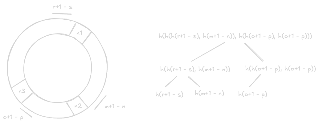
- we can handle permanent failures using “merkle trees”
- the replicas can synchronize with each other using merkle trees
- this technique is also called “anti entropy”
- the hashes of the values are stored in the leaves
- the hashes of the children are stored higher up
- if the value of a node matches, we do not need to proceed further
- if they do not match, we recursively compare the left and right children
- this technique helps detect the inconsistencies quickly / reduce the amount of data transferred
- below we show how the merkle tree for a node is constructed
- now, recall the concept of virtual nodes
- so, it has to handle multiple key ranges
- above image was for a specific key range
- below is the merkle tree for a node considering all its virtual nodes
- now, we already saw how temporary failures can be handled earlier
- in temporary failures (much more common) the nodes always come back up eventually
- so, we typically do not have to perform rebalancing of keys, recalculation of merkle trees, etc immediately
- however, in case of permanent failures, the nodes go down permanently
- so, changes in “membership” i.e. nodes getting added / removed from the cluster need to be communicated
- naive approach - every server communicates to every other server
- disadvantage - not scalable due to all permutations of connections
- better approach - communication using “gossip based protocol”
- every node has some nodes in its “token set” and communicates the changes to it
- e.g. node a has (b, e) in its token set and communicates the changes to it
- node e has (c, d) in its token set and communicates the changes to them
- this way, all membership changes are communicated throughout the cluster “asynchronously” / “eventually”
DynamoDB
- difference from key value store - this is more towards “multi tenancy” / more towards a key value store as a managed service by a cloud provider. so, this has concepts like adaptive, bursting, etc
- “multi tenancy” - load of one customer should not impact another i.e. if one customer has a sudden spike in traffic, it should not impact the other customers
- no cap on table size - tables can have trillions of rows as well
- dynamo db has a collection of tables
- each table has a collection of items
- each item is uniquely identified by a “primary key”
- the primary key needs to be specified during table creation
- primary key is composed using two parts - “partition key” and “sort key”
- partition key is required. it determines which partition the item goes to
- sort key is optional i.e. if not provided, partition key becomes the primary key. it determines how data is stored within a partition
- supports “secondary indices” - useful when we want to query using an attribute that is not the primary key, as otherwise our queries would go through a full table scan. e.g. if we want to query using the age attribute of a user instead of the user id, we can do so. how it works internally - this secondary index is also a dynamo db table itself! the primary key is the age attribute (i.e. the column we want to index on), while the value is the user id (i.e. the primary key of the original table)
- a “data node” is responsible for multiple “partitions” across different tables
- “partition abstraction” - dynamodb works using the partitions of the tables, and not the tables or data nodes directly. e.g. algorithms like raft / paxos (dynamodb uses multi paxos) work at partition level, and not at table / node level. advantage - if a partition is becoming hot, it can easily be split into multiple partitions and redistributed across multiple data nodes
- writes go to the “primary” / “leader” replica partition
- “strongly consistent reads” go to the primary replica, while “eventually consistent reads” can go to any replica
- how writes work -
- writes go to the leader replica first
- the leader writes it to its wal (write ahead log file) synchronously
- it then communicates it to the other replicas for replication
- the replicas too write it to their wal files
- finally, the leader replica acknowledges the write to the client
- understand how all this writing to wal files was synchronous
- now, all the data nodes asynchronously write the data from their wal files to the actual partitions
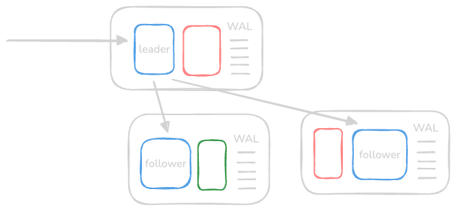
- “partitions” are composed of two things - “b trees” and “wal files”. b tree stores the actual data, while wal files store all the write operations
- replicas can be of two types -
- “storage replicas” - same as the partition described above
- “log replica” - contains only the wal file, and not the b tree. advantage, my understanding - replicating a log replica is easy, as we can continue accepting writes, while the b tree is getting replicated in the background. so, it can be used for backups etc
- “metadata service” - stores the mapping of partition to data node
- flow of operations -
- client requests reach the router
- the router fetches the data node for the primary partition from the metadata service
- the router then forwards the request to the data node with the primary partition
- this replica writes to wal / replicates it to the secondary replicas
- after the replication, the client receives the acknowledgement
- the metadata does not change often. so, the router “caches” the metadata. note - we are caching the metadata, and not the data itself
- “storage admission control” - ensures data nodes are not overwhelmed with requests
- when creating a table in dynamodb, we configure rcu / wcu (“read / write capacity units”)
- so, we need to ensure that if for e.g. the customer pays for 300 rcu, they cannot make more requests than that
- a data node has partitions from different tables. e.g. assume a data node has partition 2 from table 1, partition 3 for table 2 and partition 1 for table 3. now say the data node is capable of handling 1000 rps. the storage admission control needs to ensure that the sum of capacities of all the 3 partitions mentioned above does not cross 1000 rps i.e. the capability of the data node they are on
- problem - “throughput dilution” - assume the following scenario -
- there is a hot partition
- we had x partitions initially
- dynamodb scales up to x+1 partitions to handle this hot partition
- assume we provisioned q rcu for the table
- while each partition would initially be allowing q/x rps, it would now allow q/(x+1) rps
- problem - what if the partition was hot due to a specific key (e.g. taylor swift tweeted something)?
- the same key that was initially part of the partition allowing q/x rps would now allow only q/(x+1) rps
- solution 1 - “bursting” -
- not all partitions of a data node would use all the capacity at the same time
- so, we allow the hot partition to use the unused capacity of the data node temporarily
- implementation - “token bucket algorithm”
- each partition has two buckets - one for the “provisioned capacity”, and another for the “burst capacity”
- so, even the bursting has an upper limit like provisioned because of this bucket
- solution 2 - “adaptive” -
- bursting is useful when the spike is short lived
- but what if the spike is long lived
- e.g. scenario - our partition key is time. partition for the last hour will receive the most rps as compared to the other older partitions
- so, we want to be able to support the following use case - say the wcu provisioned by customer is 1000. there can be 2 partitions, one receiving 800 rps, while the other receiving 200 rps
- there are “global token buckets” in the storage admission control
- if the global token bucket has tokens, the partitions can use more than their provisioned capacity
- so, instead of tracking at a partition level, we track the rps at table level here
- so, the new flow is now as follows -
- the router first requests the storage admission control to ensure that the client is not exceeding the request limit at the table level
- then, it sends the request to the right partition using the metadata service
- now, we have handled adaptive. now, techniques like bursting, ensuring requests for a data node does not exceed its capacity, etc are handled at the partition level as before
- idea is we never stopped accepting writes (availability). now, the actual write to the bst can be delayed. this means we are sacrificing most up to date reads (consistency)
- durability - using wal files, log replicas, etc as discussed earlier. these wal files can also be archived to s3 periodically for durability
- this archiving to s3 helps with not only backups, but can help with cross region replication, and even cdc (change data capture) flows using “dynamodb streams”
- we use checksums when reading / writing data to ensure integrity
- lot of aggressive testing - injecting failures, chaos monkey (end to end testing), “canary deployments” for new features, etc
Metadata Caching
- engineers at amazon are against variance
- better that a page loads every time at 40ms, rather than sometimes at 10ms and sometimes at 200ms
- recall how the request router is getting the data from the cache
- this cache is in the user’s “critical path”
- amazon observed a hit rate of 97.5% on this cache
- what if there is a failure / router service restarts?
- all the requests will now go to the metadata service - since the cache is ephemeral
- this can overwhelm the metadata service
- so, amazon keeps calling metadata service asynchronously in the background
- this way, it not only keeps updating its local cache in the background, but also prepares the metadata service in case of an outage in the router service
Content Delivery Network
read this, it covers basics, push and pull, etc
Components
- “clients” - end users like browsers, smartphones, etc that request for content from the cdn
- “routing systems” - direct clients to the nearest cdn facility
- “scrubber servers” - separate good traffic from malicious traffic, against popular attacks like ddos
- “proxy servers” - serve “hot content” from ram, while they can also have “cold content” on disk / ssd
- “distribution system” - distribute content to all the edge proxy servers
- “origin servers” - cdn fetches unavailable data from origin servers and serves them to the clients
- “management systems” - track usage, latency, statistics, etc. useful for optimizing cdn, billing customers in case of third party cdn, etc
Workflow
- the “origin servers” first tell about their “uri namespaces” to the “routing systems”
- uri namespace means how the content is structured in a hierarchy, e.g. /images/products/nike-123.jpg
- the origin server then publishes its content to the “distribution system”
- the “distribution system” in turn distributes it to the edge “proxy servers”
- after this, the “distribution system” informs the “routing system” about what content is cached on which “proxy server”. this helps the “routing system” route the traffic to the right edge “proxy server” efficiently
- the “client” requests for content to the “routing system”, which returns the right “proxy server”’s ip address
- after this, the client calls the “proxy server” using this ip address
- but first, it goes through “scrubber servers” for filtering out malicious traffic
- then, the request reaches the “proxy server”, which returns the actual content
- the “management system” continually monitors various metrics which can be later used to optimize our cdn
- when the request reaches the “proxy server”, it will first check locally. if it not available, it will probe the remaining “proxy servers” in its pop (point of presence) for the content
- alternatively, each pop can maintain its datastore around what content is available on which proxy server
Dynamic Content Caching Optimization
- we can execute scripts at the edge proxy server to avoid making requests to the origin server
- e.g. updating with information like the weather, timestamp, etc
- this is also called “esi” or “edge side includes” markup language
- only small portions of the webpage change. fetching the whole webpage for this makes no sense
- so, esi helps specify which portion is changed, so the rest of the portion of the webpage can be cached
- the dynamic portions are assembled on either the edge proxy server or on the client browser
Multi Tier CDN Architecture
- the “proxy servers” are typically organized in a tree like structure
- this reduces the burden on the origin server (or distribution system in our case), as it does not have to distribute the content to all the proxy servers
- the parent edge server at the point of presence distributes to its “peer” child edge servers easily
origin server - edge server - edge server | |- edge server | |- edge server | |- edge server - edge server |- edge server - another advantage apart from effective distribution - “tail content”
- research shows that only some content is popular, the remaining content is rarely accessed
- multiple layers of cache helps handle this as well
- tail content can be kept in for e.g. parent edge servers
- the child edge servers can ask parent edge servers for tail, less frequently accessed content
- the child edge servers contain the most frequently used content only, which serves 99% of the use cases
- the child servers are smaller in size and much more in number, while the parent servers are much more computationally capable but much lesser in number
Routing System
- approach 1 - “client multiplexing”. return the list of candidate ip addresses to the client to choose from
- disadvantage - the client lacks the overall context
- there are multiple factors that help determine the nearest proxy server -
- network related concerns like number of hops, bandwidth limits on the path, etc
- being in the same or closer geography
- load a proxy server can handle - if a proxy server is overloaded, forward the request to a location with significantly lesser load
- my understanding - first, there is a “dns redirect”. e.g. if we request for video.example.com, we are redirected to cdn.example.com i.e. the original url is for the origin server but gets redirected to the cdn
- this way, we will now reach the authoritative name server of the cdn instead
- “anycast” is used i.e. all edge servers in different geographies have the same ip address
- it can factor in the various parameters we discussed above like latency, geography, etc
- the protocol used in anycast is called “bgp” or “border gateway protocol”
- the ttl is generally kept short. this way, we are forced to make new dns requests quicker and we are routed to possibly a different proxy server, thus avoiding overloading of a single server
Consistency
- “periodic polling” is used by the “pull model” to avoid the data at the proxy servers being stale. the time duration is called “ttr” or “time to refresh”
- issue with ttr - it consumes unnecessary bandwidth for data that is infrequently changing
- so, we use “ttl” or “time to live” instead
- the same content is served to the clients till ttl. after that, the origin servers are checked for the data
- if it has changed, the updated data is fetched and served. else, the ttl is reset
- the third method is using “leases”. lease is the duration for which the origin server agrees to notify the proxy server if the data changes
- once the lease duration expires, the proxy server requests for a fresh lease
- based on monitoring, the lease duration can be determined dynamically. this is called an “adaptive lease”
- fourth method - “entity tags” or “etags” - when content is initially fetched, an etag is also provided
- this etag references the version of the content
- the subsequent requests to the origin server provide this etag under the header “if-none-match”
- if the etag matches, the origin server returns a “304 not modified response”
- however, if the etag does not match, the new updated content is returned along with the new etag
Deployment
- two places where we can deploy the proxy servers -
- “off premise” - at the isp (internet service provider) directly
- “on premise” - in data centers of the cdn provider
- off premise works usually, but would not for cases like youtube, where we have such huge amounts of data that is continually expanding as well
- so, we can use a hybrid approach based on our use case - deploy some proxy servers off premise, while the rest on premise
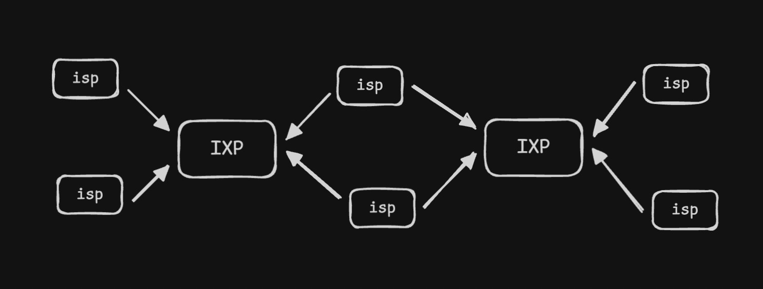
- “ixp” or “internet exchange point” - junction between isp. its a place where different networks connect and exchange traffic
![]()
- so, we use “split tcp” - clients use tcp for client to ixp. then, low latency, already established tcp connections are used for ixp to cdn communication
- if the clients were to connect to the on premise directly, there would be a lot of latency due to the longer distance, the three way handshake, etc
- this split helps us optimize the performance by a lot
- above, we discussed where to deploy cdn servers. now, how do we decide how many proxy servers we need to install, in what pop, etc?
- we need analytics for this. tools like “proxy teller” can also help us with this
How CDNs are Used
- most companies use cdn providers like akamai, cloudflare, fastly, aws cloudfront, etc
- bigger companies build their own cdn solution. e.g. netflix built “open connect”
- this helps them address security related concerns, truly optimize the infrastructure for their use case, etc
Sequencer
Use Cases
- millions of events happen in a large distributed system like twitter. we want to assign a unique id to each of these events to differentiate between them
- assigning a primary key to an entry in databases. the inbuilt auto increment feature would not work if our database is for instance horizontally shared
- facebook’s end to end performance tracing and analysis system “canopy” uses trace ids to uniquely identify an event across the execution path
Requirements
- “uniqueness” - we need to assign a unique id to each event
- “scalability” - generate 1 billion ids a day
- “availability” - multiple events happen within nanoseconds, so we need to generate ids for them
- id length calculation - we generate 64 bits, because 2^64 / 1 billion events a day ~ > 50 million years. so, we will need more than 50 million years to deplete the identifier range
- additional requirement - make them “time sortable”
Solutions
- solution 1 - using uuids. these are 128 bits
- advantage - it does not require any synchronization, each server can generate its own uuid
- it is scalable and available as well
- disadvantages - its 128 bit and not 64 bit
- it can be slow for an index (due to the extra bits)
- additionally, it has chances of duplication (though less), and is not absolutely unique
- additionally, uuids need not be monotonically increasing
- note - we can use hex strings instead of numbers, but strings are not as efficient as numbers
- solution 2 - we use a central database that uses auto increment
- all the different servers request this central database for an id
- disadvantage - single point of failure
- so, we modify it instead to have multiple database servers, and increment values by m, where m is the number of different database servers in our clusters. this helps avoid the collision
- now, each database server increments by m
- e.g. server a goes 1, 4, 7…, server b goes 2, 5, 8…, server c goes 3, 6, 9…
- downside - adding or removing servers in case of failures is not easy. e.g. one server fails, and m becomes 2. now, server a generates 9 next, which was already generated by server c
- solution 3 - we use unix timestamp (one per millisecond)
- for scalability - we can have multiple servers, and append server id to the timestamp
- disadvantage - same id will be assigned to two concurrent events occurring at the same millisecond. assume the id request for both goes to the same server (so that server id is the same as well)
- solution 4 - using a “range handler”
- we have a central server that provides a range when requested. e.g. 1 - 1,000,000,000 then 1,000,000,001 - 2,000,000,000 and so on
- the servers ask for ranges the first time / when they run out of ranges
- there are no duplicates - each microservice can respond to requests concurrently
- this range handler can have its own replicated database to track which ranges are available, which range was assigned to what microservice, etc
- the range server can have a failover server for fault tolerance
- cons of this solution - we loose significant ranges when the service dies, and have to provide a new range. solution - allocate shorter ranges to the services, but it should be large enough to serve identifiers for a while
- another con - causality is not maintained when using this solution. i am guessing this is happening because we are not maintaining any component for time in this case
- e.g. now, assume we want to bring multiple data centers up to handle increasing requests. we now will have multiple range servers. how to handle this? “geographic sharding”. my understanding - it basically means that each data center will have its own “range handler”
Causality
- we ensured generation of unique ids here
- we want to display “causality” somehow
- assume john replies to peter’s comment - these are dependent / non concurrent events
- assume john and peter reply to separate posts - these are independent / concurrent events
- having this causality also helps implement strategies like “last write wins” (discussed in databases)
- time can be used to help with causality because if for e.g. some event occurred at 6am, and something else at 7am, we can say that the event at 6 am happened first
- next, we discuss the solutions for causality
Twitter Snowflake
- we break the 64 bit into the following components -
- 1 bit for sign - we always assign a 0. this ensures we only have positive integers
- 41 bits for time - assume we want millisecond precision. this means we get ~ 70 years. the idea is that we have our own version of epoch (e.g. january 1, 2025), and we can go upto 70 years from that point
- 10 bits for worker id - so we can scale upto 1024 workers
- 12 bits for sequence number - so, we can generate upto 4096 ids per millisecond. we will start throttling if we have to generate more till the next millisecond comes
- cons of this solution - “dead period” i.e. a lot of ids are wasted with this approach when no ids are generated
- another con - “physical clock” for timestamp. there can be errors of magnitude of seconds with physical clocks, and we can have duplicates when we have multiple horizontally scaled workers generating ids
Monitoring
- “logging” - servers write metrics to a file
- advantage - absorb any momentary spikes, by decoupling the data generation and monitoring systems
- however, it can be relatively slower to process, and we might want to react faster
- additionally, logging is scoped to individual servers, unlike a centralized monitoring solution, which for e.g. helps us look at the “correlation” between failures. this is why we need a centralized solution
- “centralized monitoring systems” - an automated way to detect failures in distributed environments
- “downtime cost” - problems in one service, e.g. automated upgrades can cause problems that can quickly snowball into much large problems, if not corrected immediately
- we divide monitoring to focus on “server side errors” and “client side errors”
- “server side errors” - occur on the server, 5xx in response status codes
- “client side errors” - occur on the client, 4xx in response status codes
- “metrics” - what to measure in what units, e.g. network throughput in megabits per second
- we need to track how many physical resources our operating system uses, e.g. cpu stats like cache hits and misses, ram usage by processes, page faults, disc read and write latencies, swap space usage, etc
- there are two strategies to achieve for “populating metrics” - “push” and “pull”
- “pull” - the “monitoring system” asks the system for its metrics. the system just needs to expose its metrics via an endpoint
- advantages of pull -
- monitoring system can pull the data on its own schedule without being overloaded by systems sending too much data
- it does not require installing daemons on every server to push these metrics
- “push” - the “distributed data collectors” send their collected data to the “monitoring system” periodically
- advantages of push -
- when a firewall prevents the monitoring system from accessing the server directly
- it is more realtime than the pull strategy
- we use “time series database” to persist metrics
- tsdb helps store timestamped data like sensor readings, stock prices, etc
- some tools help convert relational databases into tsdb, but now we also have solutions like influxdb
- they are optimized for time based indexing and querying, performing aggregations over intervals, etc
- “code instrumentation” - add code to our applications for logging and monitoring information
- “alerting” - it has two parts - “take an action” when the metric values breach a “threshold”
Server Side Monitoring
- requirements -
- monitor critical processes on a server for crashes etc
- monitor anomalies and overall health of cpu, memory, average load, etc
- monitor hardware components like slowed disk writes, power consumption, etc
- monitor infrastructure like network switches, load balancers, etc
- monitor network e.g. latency on paths, dns resolution, etc
- now, we will discuss the design part of it
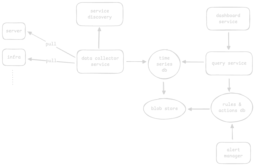
- “time series database” - store metrics data like cpu usage
- my understanding - the services interact with the time series database using queries like show me the error transactions for the last hour. the time series uses a “blob storage” underneath and abstracts it away from us. this way, the data collector can write to / query service can read from it, without worrying about the internals
- the “data collector” pulls metrics from the services it has to monitor (both software and hardware)
- “query service” to query the metrics of the time series database
- we use “distributed logging component”. recall how it uses a distributed message queue underneath
- the messages can have the following parts - service name, ids and the log
- my understanding - on one hand, the data collector can poll relevant metrics from the different systems / services, while on another hand, the distributed logging approach can be used for collecting logs and events from those systems. this might be needed maybe because logs have much more volume
- we use a “pull strategy” for the data collector. advantages of push and pull over each other were discussed here
- “service discoverer” - helps data collector determine the services to monitor dynamically
- “rules and actions database” - store rules like generate an alert when cpu usage exceeds 90%
- just like the time series database, it too can use the blob storage underneath to store configuration and abstract it away from us
- “alert manager” - send notifications via slack on violations of rules. it interacts with the rules and actions db
- “dashboard service” - displaying the data. it interacts with the query service
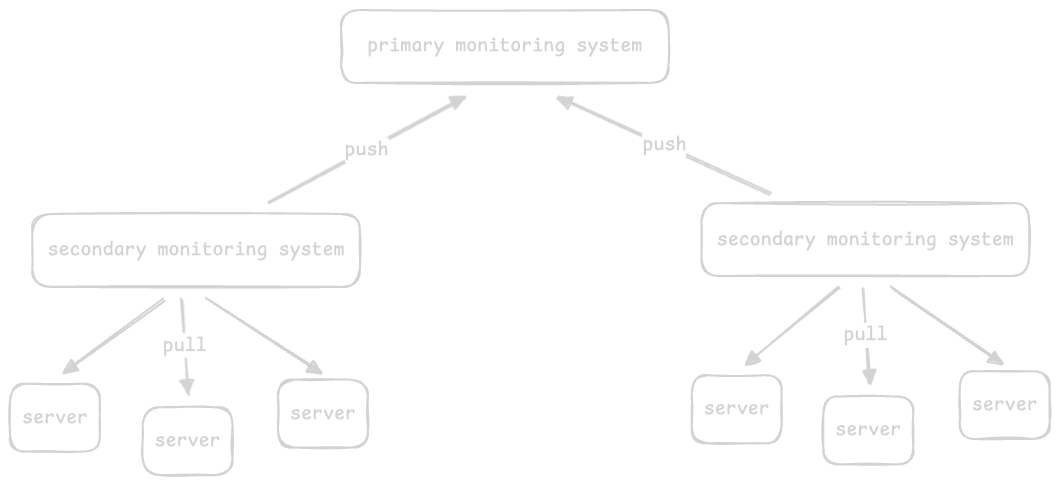
- issue 1 - the single monitoring system is a point of failure. we can use a failover server. however, while it solves the single point of failure issue, it does not scale well, specially given the volume of monitoring data
- issue 2 - given the enormous amount of data, we want to delete old unwanted data periodically to utilize the resources efficiently
- one way to scale effectively is by using “hierarchy”
- so, we have a secondary set of monitoring services that use the pull based approach, e.g. we have a monitoring system per 1000 servers
- then, we use a push based approach for pushing data from the secondary monitoring services to a global primary monitoring service
- secondary monitoring systems act as a buffer if the primary monitoring system goes down. this is called as the “offline approach”, and is also typically used in large distributed systems
- for the second issue, we use “blob storage” to store raw, excessive and expired data, while the databases like elasticsearch, tsdb, etc are highly optimized for deriving insights quickly
- we can use “heat maps” to easily identify problems among thousands of servers
- each server is named and sorted by data center, then cluster, then row
- we can use colors like green / yellow / red to show their health status
- e.g. if a row is orange, it would mean there is a potential issue in the row of racks of servers. we need to go to the data center and investigate the specific row

Client Side Monitoring
- very important point - they are much harder to track - since the error does not happens on our servers
- some examples - dns name resolution failure, failure in cdns, etc
- approach 1 - we run small services called “probers”
- these probers try to mimic user behavior
- we place them on various parts of the globe
- it periodically sends requests to check our service’s availability
- disadvantage 1 - it is not a true representation of the typical user behavior
- disadvantage 2 - having good coverage across all regions is very expensive
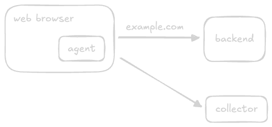
- improved solution - instead of placing them separately, we embed the “probers” inside the user applications themselves. we can call them “agents”
- now, we have the “collector” / monitoring service
- again, we can use the same hierarchical structure we discussed above to scale it easily
- but then make include some changes in the design, e.g. support for realtime analytics based on requirements - usage analytics based on geography, response times, time taken to paint the browser, etc
- “activate and deactivate reports” - clients should be able to choose between whether or not they want such reporting / monitoring to be enabled, and even have granularity over this
- as a guiding rule - we should collect as little information as possible
- “reach collectors under faulty conditions” - we should host our collector on a separate domain / ip address and even autonomous system / bgp (border gateway protocol)
- this way if there is any issue with our backend service, we can detect it easily. if they were in the same system, it would have been impossible to do so
Distributed Cache
Background
Requirements
- “functional requirements” - insertion and retrieval of data
- “non functional requirements” - availability, scalability, performance, consistency (e.g. different cache clients retrieving data from different cache servers - primary and secondary, should see the same results), affordability (use commodity hardware instead of an extensive supporting component)
- if asked in interview - answer this question from all learnings above itself
- differences from key value storage -
- “volatile” vs “non volatile” storage - cache uses ram
- geared towards performance - i feel consistency guarantees can be lesser
Considerations
- “eviction policies” - since cache sizes are small, we need to remove less frequently accessed data from it. we have various strategies like lfu, lru, mru (most), mfu, fifo, etc
- “cache invalidation” - data might become stale over time. to solve this, we use “ttl” (time to live). there are two methods for achieving this -
- “active expiration” - actively check the ttl through a daemon process or thread
- “passive expiration” - check the ttl at the time of access
- “storage mechanism” -
- use “consistent hashing” to locate the cache server in a distributed cache where the data is located
- use “hash functions” to locate the cache entries inside a cache server
- use “doubly linked list” to add or remove data. e.g. remove data from tail, relocate data to head, etc. these are all constant time operations with a dll
- “bloom filters” help determine if a cache entry is definitely not present in the cache, but the possibility of its presence is probabilistic
- “dedicated cache” - the servers the cache is stored on and the application servers are different
- advantage - flexibility in scaling, independence in hardware choice, etc
- “colocated cache” - embed cache and service logic in the same host
- advantage - reduced “capex” (capital expenditure) and “opex” (operational expenditure)
- “cache client” - perform actions like selecting the cache server to route the requests to (since data is sharded due to distributed cache), coordinate with other services like configuration service / discovery service
- note - it is not the library on the client side, but an independent horizontally scaled service. basically the flow is, client -> load balancer -> cache client -> distributed cache servers
- requests from user can be directed to any of the cache client, which abstracts away the internal complexities
- now, it can either be embedded inside the cache servers itself (if the cache is for internal use), or be run as an external service (if the cache is for external use). i think we are designing for the second purpose here
- apart from ram, secondary storage can be used to rebuild cache in case of reboots
- all cache clients are connected to all cache servers, and cache servers use non volatile storage for helping in case of failures and reboots
- we saw how the requests go via the “cache client”. how does the cache client stay updated about the addition / removal of additional cache servers?
- solution 1 - a configuration file is stored in each cache client. it gets updated about the metadata of each cache server as they join / leave the cluster
- solution 2 (better) - this configuration file is instead stored centrally
- issue with both solutions - mechanism to push updates to these files is not easy
- solution - a configuration service that maintains the data of all these cache servers. note - this feels like a “discovery service” to me
- updated flow - client -> load balancer -> cache client -> discovery service -> distributed cache servers
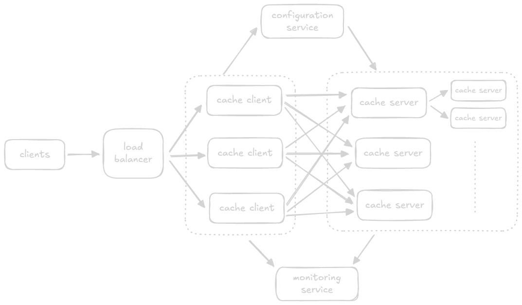
- for higher availability, we can add “replica” nodes (see the 2 small boxes above)
- to solve for inconsistency, we can use “synchronous replication” for the same data center and “asynchronous replication” for e.g. for across data centers. i feel this gives us a good balance between speedy writes, consistency and availability
- for issues like “hot partitions”, recall how we solved using “virtual nodes” during consistent hashing here
- we do not typically talk about delete, since it is typically handled using “cache invalidation” / “eviction policies”
- however, there are cases when we need it, e.g. when data is deleted from db, we would want to remove it from cache as well to remove inconsistencies
- how we can compare caching strategies -
- assume cache hit time = 5ms, cache miss time = 50ms (including access time to get from database)
- now, assuming cache hit rate with mfu is 10%, and lru is 5%
- effective access time = (ratio hit * time hit) + (ratio miss * time miss)
- so, effective access time for mfu is 7.5ms, and lru is 6.25ms
- redis and memcached comparison might come up here as well, refer this
Distributed Messaging Queue
Functional Requirements
- queue creation - create a queue with specified queue name, queue size, message size
- producers should be able to send messages to a queue
- consumers should be able to receive messages from a queue
- delete message - after processing, consumers should be able to delete messages from a queue
- delete queue
Non Functional Requirements
- durability - data received by a system should be durable, and not be lost
- availability, scalability, performance
Considerations
- naive approach - “single server message queue”, where the producer, consumer and the queue - all are on the same node
- in this, a lock is acquired when producing messages into it / consuming from it
- this helps with consistency, but degrades availability and reliability
- “ordering of messages” -
- messages in a messenger application require strict ordering. otherwise, looking at the message history can become confusing
- emails from different users does not require strict ordering
- “best effort ordering” - ordering is based on the order in which the queue received the messages
- “strict ordering” - ordering is based on the order in which the producer produced the messages
- to ensure strict ordering, we can tag messages with timestamp on the client side
- issue - it is not synchronized across different clients
- we can use a synchronized clock instead to tackle this
- additionally, we also tag them with the process identifier, in case clients on different machines produce a message at the exact same time
- note - similar approaches were discussed in sequencer
- next, the servers needs an “online sorting” algorithm, to keep the messages sorted by this timestamp as they keep coming in
- to make this approach faster - we use “time window” approach - sort the messages in a specific time frame, then add them to the queue
- my understanding - once we are confident, this time window is ready for extraction, and our system gets rid of this window
- how to handle “late messages”? because by that time, the messages after it might already have been consumed by the consumer
- in such cases, we can for e.g. put it in a special queue for the clients to handle such cases themselves
- now, to maintain strict ordering on consumer side, we need to hand out the messages one by one
- this of course affects the throughput - so ensuring strict ordering decreases the throughput as well
- now, how to manage concurrency - multiple producers producing to / consuming from the same queue?
- option 1 - using locks. disadvantage - not scalable when multiple processes keep competing for the lock
- option 2 - we use the natural buffering mechanism of os to process requests one by one
- we use a single thread to handle all operations like adding to / consuming from the queue
- so, both producers and consumers contact the same port for e.g. for their requests
- the operating system automatically processes the requests in the order in which they arrive
- this does not require any additional locks, and at the same time ensures that no race conditions occur
- notice in the diagram how the single thread is handling all requests
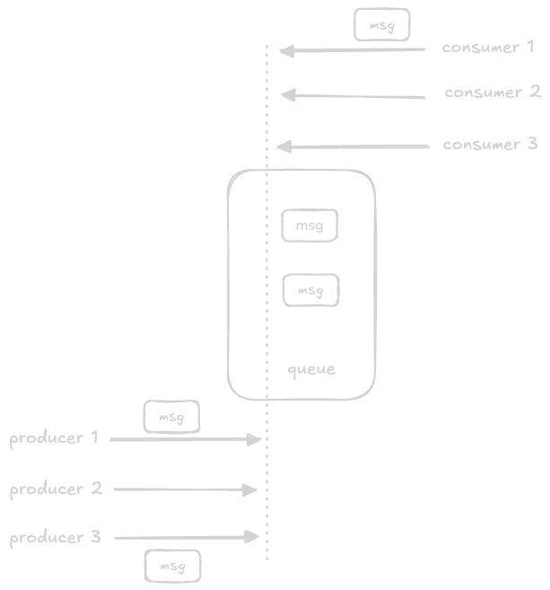
- the frontend service of producer and consumer can be maintained separately to help scale them independently - producers might have more bursty kind of workloads, e.g. handle spikes during flash sales, while consumers typically have a much more stable workload
Design
- “frontend service” - it will make appropriate calls to the metadata store / backend store
- this frontend service can also handle “request deduplication” by calculating sha of the value / by using the key we generated earlier
- it provides features like “authentication”, “authorization”, “request validation”
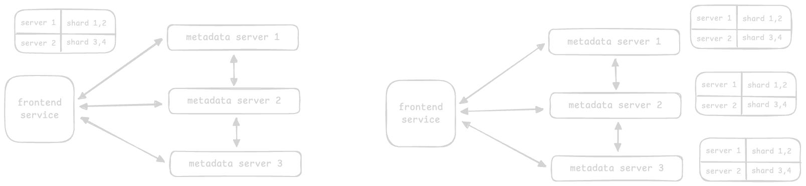
- “metadata service” - this component is responsible for managing the metadata of the queues. this can include queue names, sizes, retentions, and importantly mapping of queue name to the right backend host or cluster
- the frontend service first uses its “cache”, and if not present, it falls back to the metadata service
- there are three approaches for managing this metadata -
- approach 1 - when the metadata is small enough, the data is replicated on each metadata server, and any random server can be reached for the data via a load balancer
- what if the data cannot fit in a single machine? we use “sharding”. there are two ways to handle this
- approach 2.1 - the “mapping table” is maintained on the frontend service. the mapping table tells us which server is responsible for which shard of data. the frontend service directs the requests to the right server
- approach 2.2 - the “mapping table” is maintained on each of the metadata service servers. the frontend service directs the requests to any of the servers, and the servers themselves direct it to the right server. this approach is preferred for “read intensive” applications
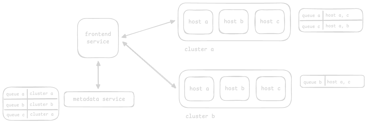
- after receiving a message, the frontend service calls the metadata service to determine the responsible hosts of the “backend service” for that particular message and queue
- due to the huge amounts of data, we can divide the backend service into “clusters”
- each cluster has its own mapping table, which tells it which nodes are responsible for which queues
- the metadata service needs a mapping table to direct requests to the right backend service cluster
- this way, we are basically able to divide the backend service itself into several clusters
- the frontend service first asks the metadata service about which cluster to direct the request to, and then directs it to the right cluster
- however, the host of the server is still chosen at random, and the redirection of the request to the right server is handled internally
- finally, it uses a “primary-secondary” model. each queue is assigned a primary node and a set of secondary nodes. writes reach the primary node and is then replicated to the secondary nodes (like synchronous replication). this architecture also means that we need a “cluster manager” like zookeeper for managing nodes for scaling, failures, etc. we also take regular snapshots for additional backup
PubSub
- distribution is push based, so consumers need not poll for new messages frequently
- key difference from distributed messaging queue - we can have multiple consumers here
- it helps handle large scale “log ingestion”. e.g. meta uses a pub sub system called “scribe” to help with analyses of user interactions
- it can also be used to replicate data between leader and follower asynchronously
Requirements
- creating a topic
- writing messages
- consumers can subscribe to topics to read messages
- specify retention time after which message should be deleted
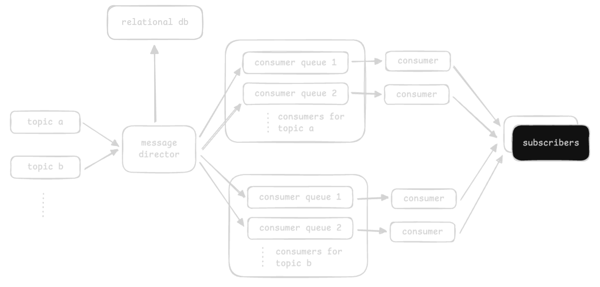
Approach 1
- we will use a relational database to store metadata like which consumers are subscribed to which topics
- why relational database - we need “strong consistency” for partition assignments, consumer offsets, etc
- we use distributed message queues for topics
- each topic would be a distributed message queue, and each consumer will subscribe to its own queue that it consumes from
- the “message director” directs data from the “topic queue” to the “consumer queues”
- disadvantage - does not scale when we have millions of subscribers for thousands of topics
- also, we are copying redundant data by duplicating it to each consumer queue
Approach 2
- “broker” - core component of our design that handles the reads and writes
- a broker has multiple topics, the topics have multiple partitions, and partitions contain messages
- each message is encapsulated inside a “segment”
- the segment contains “offsets”, which helps identify the start and end of messages
- this way, consumers can consume messages from a specific partition, from a specific offset
- each consumer can start consuming from its own specific offset
- partitions help scale the topic. producers write data to a topic, and a partition is chosen using round robin
- partitions of a topic are present on several brokers for fault tolerance
- we use local persistent storage instead of s3, due to low latency / high performance. traditional hard disks have high performance when we write to / read from “contiguous” tracks. we use “append based” writing
- for ensuring strict ordering between messages, we can support writing to a specific partition of a topic, and the producer writes all its messages to the specified partition
- “cluster manager” - it will handle the following concerns -
- maintaining the “topic registry”
- maintaining the “broker registry”
- managing “replication” for a topic and its messages across brokers
- “consumer manager” manages the consumers
- it will manage the offsets for each consumer. think acknowledgements etc as well
- it will handle not seeing of messages after the retention time
- it will allow both approaches - consumers can poll for messages, or it can also push the latest messages
Rate Limiter
Requirements
- limit the number of requests a client can send in a time window
- make the limits configurable
- client should get notifications on this breach
- availability, scalability
- types of throttling -
- “hard throttling” - put a hard limit on the no. of requests. when a request exceeds the limit, it is discarded
- “elastic / dynamic throttling” - number of requests can exceed the predefined limit if the system has excess resources. so, there is no upper limit as such
- “cgroups” or “control groups” - linux systems provide this kernel feature. available for resources like “cpu time”, “system memory”, etc. features like “resource limiting” (impose restrictions to not exceed the usage), “accounting” (monitor resource usage for billing purpose), etc
- the rate limiter can be placed in 3 places - at the client side, on the server side and as a middleware
- while some rate limiting logic can be embedded inside “load balancers” themselves, they do not have the granularity to enforce limits on individual requests based on their complexities
- the rate limiters can either be overall, or scoped to a specific user, based on the use case
- disadvantage of using rate limiter at load balancer - load balancers are typically unbiased, but our application might need granularity in terms of which endpoints need how much rate limiting depending on the kind of operation
Design
- the request reaches the “web server”
- it asks the “rate limiter” if the request should be allowed
the rate limiter can be configured using config files, e.g. lyft
domain: messaging descriptors: - key: message_type value: marketing rate_limit: unit: day request_per_unit: 5- “rules database” - store the rules. used with “rule cache” to improve performance
- “rule retriever” - updates the “throttles rule cache” when updates are made to “rules database”
- “throttles rule cache” - the cache consists of rules in rules database. it helps serve requests faster than persistent storage
- “decision maker” - make the decision based on one of the algorithms
- “client identifier builder” - generate a unique id for the client using ip address, login id, etc. notice how we cannot use a general sequencer here, because we want to be able to identify the client accurately
- so, the entire flow is as follows - client request -> client identifier builder -> decision maker -> retrieve rules from rule cache -> accept request (forward request to the servers) or reject request (use of the strategies below)
- one of the two strategies can be used - “drop” or “queue” for later processing
- apis return the status code of 429 - too many requests
- what to do if the rate limiter is down? - default should be to accept the request, given the various other rate limiters like the ones at load balancers are functioning
- approach 1 - we use a centralized database
- advantage - clients cannot exceed the limits
- disadvantage - not scalable - lock contention in case of highly concurrent requests
- approach 2 - using a distributed database, where each node tracks the rate limit
- disadvantage - the client could exceed the limit while the state is being synchronized across these multiple rate limiter nodes
- “get then set” approach - retrieve the counter, increment it and finally set it back in the database
- “race condition” - e.g. when the “get then set” approach is used, if multiple requests are processed simultaneously, they all see and set the same values, making the counter invalid and bypassing the rate limiter
- solution 1 - use pessimistic locking. disadvantage - this can lead to performance bottleneck
- solution 2 - “set then get” i.e. setting the value in a very performant manner. such atomic operations with low latency requirements can be performed using redis
- solution 3 - divide the quota into multiple servers, and divide the load between them, aka “sharded counters”
- each server in this case will have a lower limit than the overall limit. each node maintains its own state, which need not be synchronized with each other
- we can use “sticky sessions” so that requests from the same client always end up reaching the same server in this case
- “online” vs “offline” updates - if the request is below the rate limit, first allow the request, so that the “web server” can then contact the “api server”. in the second phase, we update the database with the new count i.e. “offline”. this has significant effect on the performance, as we avoid computations on the client’s “critical path”
Algorithms
- “token bucket algorithm” - analogy - a bucket is filled with tokens at a specific rate
- the bucket also has a certain capacity
- the algorithm checks for a token to be present in the bucket for every request
- once all the tokens are consumed, further requests are rejected
- so, four parameters - “bucket capacity” (c), “rate limit” (r), “refill rate” i.e. duration after which a token is added (1/r) and “requests count” i.e. number of incoming requests (n)
- advantage 1 - handle bursts in traffic
- advantage 2 - memory efficient algorithm to implement
- disadvantage - surpass the limits at edges. e.g. assume refill rate is 0.33 minutes and capacity is 3. at the end of a minute, we have 3 tokens. assume after this, we receive 3 requests that are processed. then, at 1.33 minutes, a new token gets added. assume this gets consumed as well by a new request. so, we now essentially had 4 tokens consumed in around 0.33 minutes. however, i feel we saw handling of this burst as an advantage as well
- “leaking bucket algorithm” - instead of filling the bucket with tokens, we fill it with requests
- the leaking signifies the “constant rate” at which the requests are processed
- the requests might come in at a variable rate, but they are processed in a constant rate
- it might use fifo - first in / first out
- disadvantage - cannot handle bursts in traffic since recent requests can be stuck
- a client has to send 18mb data at 6 mbps. the server can process the data at 4mbps. what should be the size of the bucket?
- time taken to transfer the entire data = 18/6 = 3s
- amount of data processed in 3s = 12mb
- bucket size = 18-12 = 6mb
- “fixed window counter algorithm” - divide the time into fixed intervals called “windows”
- and assign a counter to each of window
- when a request is encountered, increase the counter of the window by one
- once the counter reaches the limit, discard the remaining requests for that window
- disadvantage - significant bursts can occur. assume we are allowed 10 requests every 30 minutes. now, assume we receive 10 requests in 25-30 minutes, and 10 requests for 30-35 minutes. while all of them are permitted, we basically had 20 requests in 10 minutes, which is significantly higher than the allowed limit
- “sliding window log algorithm” - it addresses the boundary problem we saw above
- logs are kept sorted based on the timestamp
- e.g. a request arrives at 1.00pm. the window becomes 1.00pm-2.00pm
- another request arrives at 1.20pm. as the log size is less than the maximum rate limit, it is allowed
- another request arrives at 1.45pm. the request is rejected, since the size becomes 3 which crosses the limit
- another request arrives at 2.25pm. the request is accepted, and the window is updated from 1.25pm to 2.25pm
- disadvantage - more overhead in terms of memory etc
- “sliding window counter algorithm” - combines the best of both the worlds i.e. “fixed window counter algorithm” and “sliding window log algorithm”
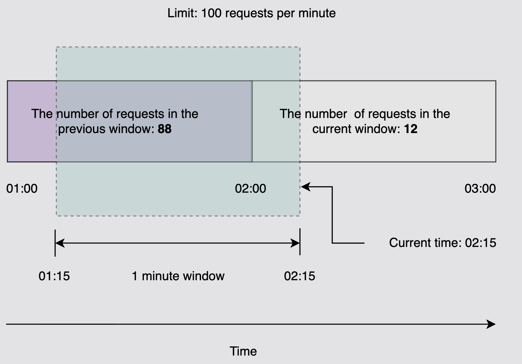
- e.g. assume that the current time is 2.15
- assume the previous window 1-2 had 88 requests and current window 2-3 has 12 requests
- so, our “effective window” becomes 1.15-2.15, and it has (88*45/60 + 12) = 78 requests, which is < 100 requests
- so, we allow the incoming request at 2.15
- final note - we can use locks with the above algorithms, if there is little lock contention. but if the lock contention is high, we need to use approaches like sharding, using finer grained locks, etc
| algorithm | space required | burst handling |
|---|---|---|
| token bucket algorithm | low | yes, within limits |
| leaking bucket algorithm | low | no |
| fixed window counter algorithm | low | yes, but can exceed limits as well |
| sliding window log algorithm | high | yes, but smoothens out the traffic as well |
| sliding window counter algorithm | medium | yes, but smoothens out the traffic as well |
Blob Storage
- for “unstructured data” like images, audio, videos
- data is stored as a “blob” or binary large object - collection of binary data stored as a single unit
- mostly, used by applications following “worm” (write once, read many)
- we cannot modify files - we can only upload newer versions of them
- e.g. youtube uses google cloud storage. it stores > 1pb of data per day. it has to store the same video replicated multiple times for availability, store the same video in multiple resolutions, etc
Functional Requirements
- create “containers” - to group blobs, e.g. store blobs for different users in different containers. then, a user can have one container for images, one for videos and so on
- “delete container” and “list containers”
- “put data” to containers. this should generate a url
- “get data” using the generated url
- “delete data”. also support “retention” (users want to keep their data only for a specified amount of time)
- “list blobs”
- “consistency” - “strong consistency” - different users should see the same view. “eventual consistency” - updates should propagate asynchronously, e.g. update to a profile picture should take time to reflect
Non Functional Requirements
- number of daily active users - 5mil
- capability of the blob store server = 500 rps. note - recall how we saw here that a 64 core server can handle 64k rps. but since a blob store involves io intensive operations, it needs 500rps instead
- average video size - 50mb
- average thumbnail size - 20kb
- number of video uploads per day - 250k
- number of read requests per day per user - 20
Calculations
- so, no. of servers = (rps) / (one server’s rps) = 5mil / 500 = 10k servers. notice how we assume all users access our service concurrently at the same time, to design for the worst scenario
- total storage = (no. of videos) * (storage per video and thumbnail) = (250k * (50mb + 20kb)) ~ 12.5tb
- incoming traffic or bandwidth required for uploading videos - (total storage per day) / (24 * 60 * 60) = 0.14 gbps
- outgoing traffic or bandwidth required for downloading videos - (daily active users * no. of requests per day * data size) / (24 * 60 * 60) = (5mil * 20 * 50mb) / (24 * 60 * 60) = 58 gbps
- note (my understanding) - in bandwidth calculations, people tend to use bits per second instead of bytes per second. so, the to numbers above can be multiplied by 8 when answering in interviews as well
Components
- “rate limiter” - limit the number of requests and “load balancer” to distribute the load
- “frontend servers” receive our requests
- “data nodes” - hold the actual data. a blob can be split into “chunks”, and a data node can hold some of the chunks of a blob
- “manager node” - manage the data nodes. e.g. track how much space is there on the data nodes etc
- note - manager nodes can become a single point of failure. so, we use “check pointing” / take “snapshots” at frequent intervals, so that these can be used to restore from the point we left off
- “metadata server” - it stores “container metadata”, “blob metadata” (which blob is stored where), etc
- “sequencer” to help generate unique ids
Workflow
- client generates a request to write
- it goes through rate limiter, load balancer, frontend server and finally the manager node
- the manager node generates a unique id using the sequencer
- the manager node then determines the space available on nodes, and returns the “chunk to data node mapping” to the frontend server. this is called a “free space management system” - the idea is to score azs or nodes which have free space. there can be other factors like depending on storage class, determining the kind of servers we should use etc
- the frontend server then performs the upload to the various data nodes
- internally, operations like replication, calculation of sha, etc happen
- finally, the id is returned to the client
- “reading” - the frontend server requests for the metadata from the manager node
- then, the chunks are downloaded from the data nodes
- parallel fetching of chunks can be performed for higher throughput
Considerations
- there are three “layers” of “abstractions” - “users”, “containers” and then “blobs”
- it helps perform routing and sharding on different levels, e.g. user id, then container id and finally blob id
- “metadata” - store chunk ids and the data nodes / replicas they are stored in
- “chunk size” can be influenced by many factors. e.g. if we use rotating disks where a sector is a unit of read / write, we should make the chunk size a multiple of the sector size
- we “group” several data nodes into “partitions”
- this way, instead of looking into all data nodes at once, we can easily locate data nodes in partitions
- “partitioning data” - if we partition data based only on blob id, blobs for a container (or say different chunks for a blob) might go into different partitions, thus making operations like list more difficult. so, we instead partition data based on the whole url i.e. combination of user id, container id and blob id
- we generate an efficient “index” using an “indexing engine”. this way, locating blobs by various attributes like user id, container id, etc becomes much easier
- we use “pagination” to in operations like “list”. the sorting of blobs can be done ahead of time in the indices we generated above, to avoid having to sort the blobs later dynamically
- “continuation token” is used to continue from where we left off
- “replication” - we perform “synchronous replication” on the read replicas of the same data center to achieve “strong consistency”. the amount of replicas is defined via a “replication factor”
- so, the synchronous replication is performed as part of the user’s critical path
- we also perform “asynchronous replication” on the replicas across regions / data centers for fault tolerance
- “erasure coding” - with normal replication, we end up consuming a lot of space. the idea is we break the data into smaller parts (say 10) and add 4 additional parity parts using some advanced mathematics. now, we have 14 parts. we store them in a distributed fashion. now, even if we loose any of the 4 parts out of these, we can still reconstruct our original blob back from the 10 parts remaining
- we use “checksums” for ensuring integrity -
- calculate and write the checksum when writing the blob
- when reading the blob, fetch it and also compute the checksum for the chunks / blob. then, verify the computed value against the actual checksum
- “data scrubbing” - it is a proactive process of identifying the corrupt data in the system and keep correcting / removing them. we can achieve this using the checksums we computed above
- “garbage collection” - when a delete request is called, it is inefficient to delete all the chunks one by one
- so, the blob is instead removed from the metadata immediately. this way, no user can now see the blob
- the “garbage collector” eventually removes the inconsistencies by reclaiming the space from the data nodes
- we can cache the metadata at various places like the frontend service, and the blobs themselves using cdns
Distributed Search
Resource Estimation
- servers required - assume we have 150 million daily active users
- assuming servers can handle 64k rps, we need ~ 2350 servers at peak load
- a single json has size 200kb - it stores video title, description, channel name, etc
- number of unique terms in it is 1000
- storage to add one term to the index is 100 bytes
- so, storage per video = 200kb + (1000 * 100 / 1000) = 300kb
- assume 6000 videos per day, total storage = 6000 * 300kb = 1.8gb
- incoming traffic - assume each search query is 100 bytes. 150 million requests per day = 1736.1 rps
- so, total incoming traffic = 0.17 MB/s (megabytes per second) or 1.39 mbps (megabits per second)
- outgoing traffic - assume we have 80 results per search, and each search result is 50 bytes. so, we need (1736.1 * 50 * 80 * 8) ~ 56 mbps
- our search results are text based, making the bandwidth modest. some searches might return thumbnails etc as well to enhance the result, thus increasing the bandwidth
Indexing
- “fuzzy search” - perform different matching queries, like finding the approximate matching strings
- searching serially through every document would be very time taking
- “inverted index” / “document matrix” - we identify the unique terms, discard the frequently occurring terms, and create a matrix
- for each term, we store the following -
- the list of documents the term appears in
- the frequency with which the term appears in each document
- the list of positions of the term in each document. notice how offsets is 2 dimensional, since a term can appear multiple times in a document
term mapping engine ([1, 2, 3], [1, 1, 1], [[9], [5], [8]]) heart ([1], [1], [[12]]) elastic ([1], [1], [[15]]) - we use the following algorithms on top of inverted index -
- “boolean” - define our searches by combining words and phrases using AND, OR, NOT, etc
- “extended boolean” - helps incorporate techniques like “term weights”, “partial matching”, etc
- “proximity” - two or more “terms” that are matching are within a certain “distance” of each other. “distance” - intermediate words or characters
- “relevance” - helps measure the accuracy between “search query” and “search results”
- this is called “full text search”, as we have some “fuzzy” logic. traditional searches would look for exact matches, which might not work for our use case
- advantage - this pre generated index makes looking up frequency of words in a document very fast
- disadvantage - “maintenance” for keeping the index up to date when adding / removing documents
- we keep the index in “ram” for low latency in searches
- our system needs to be resilient against people who try to game the system using “seo (search engine optimization) techniques”, since we only return a handful of the relevant results against a search
- if we use a centralized system for the whole process of generating and querying the index, we have the following issues -
- “spof (single point of failure)”
- “server overload” when numerous users query it
- a large index cannot fit the ram of a single machine
Design
- it has two phases - an “offline phase” for data crawling and indexing, and an “online phase” for searching for results against the search query
- “crawler” - fetches content and creates “documents” i.e. json structures
- e.g. crawl the youtube video’s channel name, title, description and possibly even the video’s annotation to help search based on content of video as well
- it then stores these documents in a distributed storage
- “indexer” - builds a searchable “index” using “map reduce” (thus getting benefits of scaling etc)
- this index gets stored in the distributed storage as well
- “searcher” - responds to search queries by running the search query on the index
- it ranks the results based on relevance and then sends the result
Indexer
- since the number of documents are huge, we need a method to “partition” this data across nodes
- we can use two techniques for partitioning this input data / documents during indexing -
- “document partitioning” - all documents collected by the web crawler are partitioned into subset of documents. then, each node performs indexing on the subset of documents assigned to it
- “term partitioning” - we obtain all terms, and divide terms into subsets. then, subsets of these terms are assigned to the different nodes
- disadvantage of term partitioning -
- imagine we want to search for the term “distributed search system”
- imagine for “distributed” we go to node 1, for “search” to node 2 and for “system” to node 3
- all three nodes return the documents that have their respective terms
- now, we need to perform a “merge” step i.e. filter documents containing all three terms
- this merge step is very expensive, as it involves transferring list of documents across nodes
- so, we use “document partitioning”
- each query is processed by all nodes, and the results from these nodes are merged before being sent to the end user
- advantage - less inter node communication is involved
- we have a “cluster manager” that manages node uptime using heartbeats, handles distribution of the documents by the document partitioning discussed above, etc
- after partitioning, the indexing algorithm is run on all the nodes to generate the inverted index on each of them
- so, we are basically storing small inverted indices on each node, instead of storing a giant large inverted index
- for search, we run queries on each tiny inverted index / node in parallel
- each node returns a “mapping list” to the “merger”
- “mapping list” - list of (documents, frequency of the term)
- the merger can perform “sorting” based on score before returning the final result to the user
- “colocation” - we are performing both searching and indexing on the same node(s)
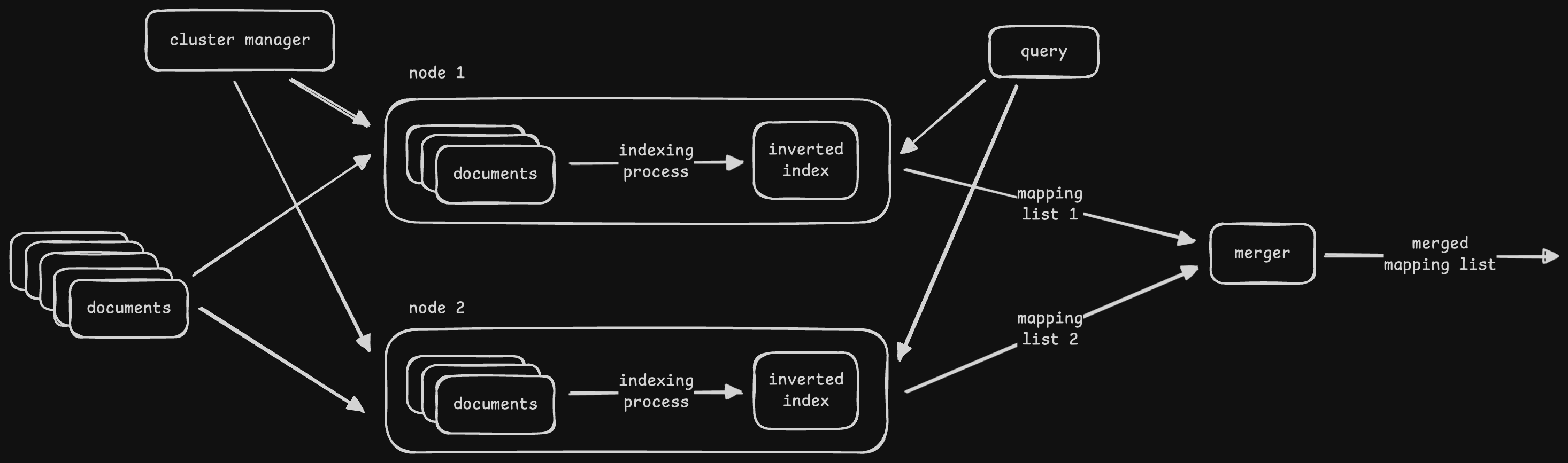
- disadvantage - we are using the same node for indexing and searching
- the two operations are different in nature, and so they have different scaling needs
- so, we introduce “distributed blob storage” between them
- we have separate sets of nodes for “indexer” and “searcher”
- first, the crawler writes the documents to the distributed blob storage
- then, the indexer reads them and writes the distributed index to the distributed blob storage
- finally, the searcher reads from the distributed blob storage to answer queries
- rest of the architecture stays the same
- since the indexer and searcher are now separated, retries, scaling, etc can be handled individually
Map Reduce
- the indexer works using “map reduce” model. below is my understanding
- recall that no. of partitions in map reduce = no. of reducers
- so basically, each reducer spits out an inverted index of its own
- each of these inverted indices can be queried individually by the “searcher” layer, thus helping with parallelism
- each mapper can go through a set of document(s) and output very small inverted indices
- the reducer takes as input these very small inverted indices, and then aggregates them and outputs relatively larger inverted indices
Caching
- “query result caching” - cache results to avoid re-computation for common queries
- “partial index caching” - cache the index (specially the frequent parts) in the ram of the searcher nodes
- cons of caching - stale data, resource overhead
Distributed Logging
- “log files” - details of events occurring in microservices
- it helps us find root cause of failures
- a distributed logging system can also help us understand user activities, which can then be input into a recommender system
- always remember to point out security concerns we should implement in systems like these -
- security at transit and at rest
- fine grained access control (authentication and authorization) and least privilege access
- masking sensitive data like ids and passwords from logs
- prevent “vulnerabilities” - e.g. the famous one in log4j in 2021 that allowed users to run malicious code
- “distributed systems” - several microservices, and each microservice has several servers. it is difficult to log into every server to view its log
- “restrain” the log size using “sampling”, as logs generated can become very huge. some examples -
- we can use sampling for logs when an application logs every time a user comments on a post
- we should not use sampling for logs related to bank / atm transactions, as they help with fraud detection etc
- “categorization” - production logs print messages with severity of “WARNING” and above. for cases where we need more detailed logs, we can use “DEBUG” or “INFO”
- we should use “structured logging” - enforcing structure helps interoperability between log readers and writers, makes the job of our distributed logging easier
Requirements
- “write logs” of the distributed system to the logging system
- “search logs” easily
- “centralized visualizer” to provide a unified view
- non functional - low latency (not affect user’s critical path), scalability, etc