Machine Learning

Supervised Machine Learning

“supervised machine learning” - labels are associated with certain “features”
a model is trained, and then it can make predictions on new features
e.g. predicting price of a car - the model learns from some “features” like mileage, make, etc, and the “target” variable i.e. the car price in this case
then, when given new data about the car, it can predict the target
so, models basically “extract patterns” from the data
“feature matrix” (X) - rows are “observations” or “objects”, columns are “features”
“target variable” (y) - a vector with the target we try to predict
the model is g. g(X) = y. the goal is to come up with g
the obtention of g is called “training”
3 types of supervised machine learning have been discussed next
“regression” - the output is a number, e.g. car’s price
“classification” - the output is a category, e.g. detecting whether an email is spam or not. it has two types - “binary” (two categories) and “multiclass” (more than two categories)
“ranking” - output is the top scores associated with the corresponding items, e.g. recommender systems

CRISP DM

“crisp dm” stands for “cross industry standard process” for “data mining”
helps us organize machine learning projects
step 1 - “business understanding” - e.g. lot of users complain about spam emails. we analyze if machine learning can help us. we think if traditional “rule based system” can be used instead, where we define rules, e.g. if the email contains the word “offer”, class it as spam. issue is manually extracting and maintaining such rules can become cumbersome in this case
next, we need to come up with metrics / a way to measure the success of our solution, e.g. reduce the spam messages by 75%
step 2 - “data understanding” - we analyze the data sources available, and decide if we need more data
step 3 - “data preparation” - we clean the data / remove noise, and convert it to for e.g. a tabular format (like the feature matrix / target variable vector) which the ml model can be fed
step 4 - “modelling” - we train the models at this step. we train different models and pick the best one. based on the results of this step, we decide if we need to add new features, fix data issues, etc. this is what the arrow back to data preparation in the diagram means
step 5 - “evaluation” - we evaluate the model’s performance, and compare it with the metrics defined in the business understanding phase
step 6 - “deployment” - nowadays, evaluation and deployment is part of the same phase, we deploy and then evaluate the model. this is called “online evaluation”. we introduce monitoring here
the project needs to be maintainable, as we might iterate over it several times

Model Selection

this is the “modelling” approach we discussed here
step 1 - we “split” our dataset into “training” and “validation”
step 2 - we “train” / “fit” the model using the training dataset
step 3 - then, the model predicts the feature matrix of the validation dataset, and the predictions are compared with the actual target variable values of the validation dataset
step 4 - we select the best model from the results above
“multi comparisons problem” - we compare the predictions of different models against the validation dataset. one of the models got lucky and predicted the validation dataset accurately
this is why, we typically split the dataset into three parts - validation (60%), training (20%) and testing (20%)
step 5 - we do an extra validation step, by running the best model from step 4 on the test dataset
step 6 - compare the metrics from the validation and test dataset

Regression

example - car price prediction. also called “msrp” or “manufacturer suggested retail price”
first, we go through the “data preparation” phase
we standardize the column names by lowercasing and replacing spaces with underscores -
```
df.columns = df.columns.str.lower().str.replace(' ', '_')
```
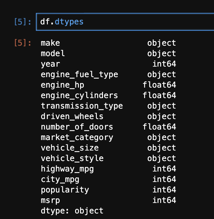
next, we try to standardize the string columns of our dataframe as well. calling dtypes on a dataframe returns us a pandas series, where the index is the column names, and the values are the types of the columns

hence, we use the below to standardize the string columns, by for e.g. lowercasing them -

str_cols = df.dtypes[df.dtypes == 'object'].index

for col in str_cols:
  df[col] = df[col].str.lower()

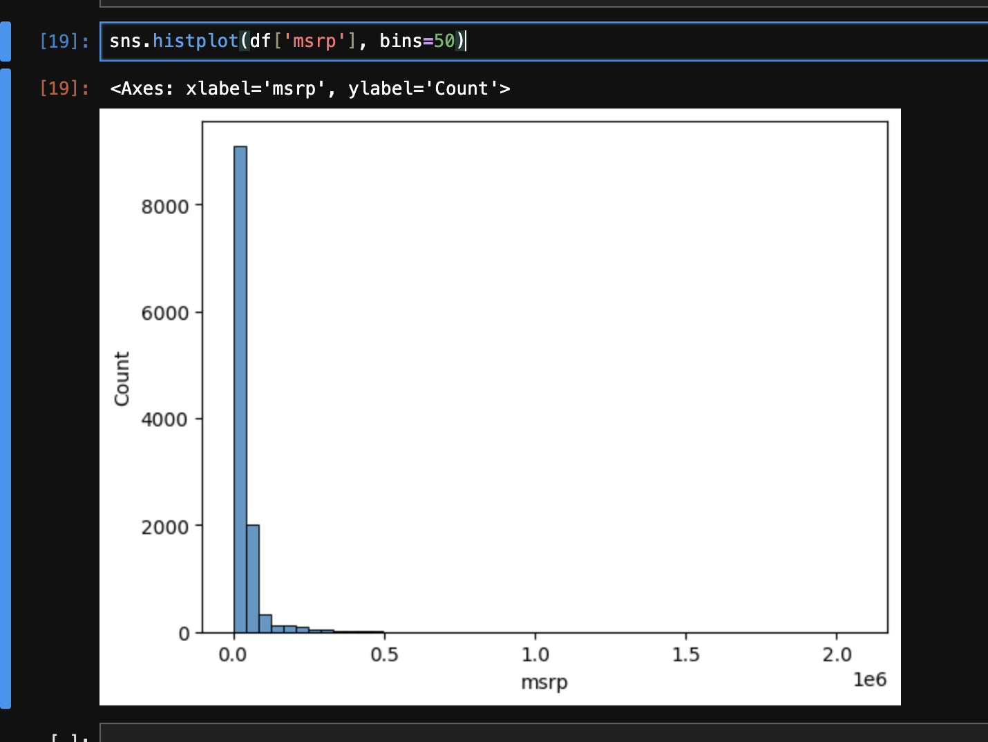
next, we perform some “exploratory data analysis”
when we try plotting the msrp, we see that its distribution is “skewed”. it is also called “long tail distribution”
we can then use some techniques to verify our thesis, e.g. by plotting sns.histplot(df[df['msrp'] > 500000]['msrp'], bins=50), we see that there are very few costly cars. this kind of distribution is not good for machine learning models
so, we apply the “logarithmic” transformation to it, as it makes the values more “compact”. it makes the distribution “normal”. see the example below to understand this -
```
np.log([1, 10, 1000, 1000000])

# array([ 0.        ,  2.30258509,  6.90775528, 13.81551056])
```
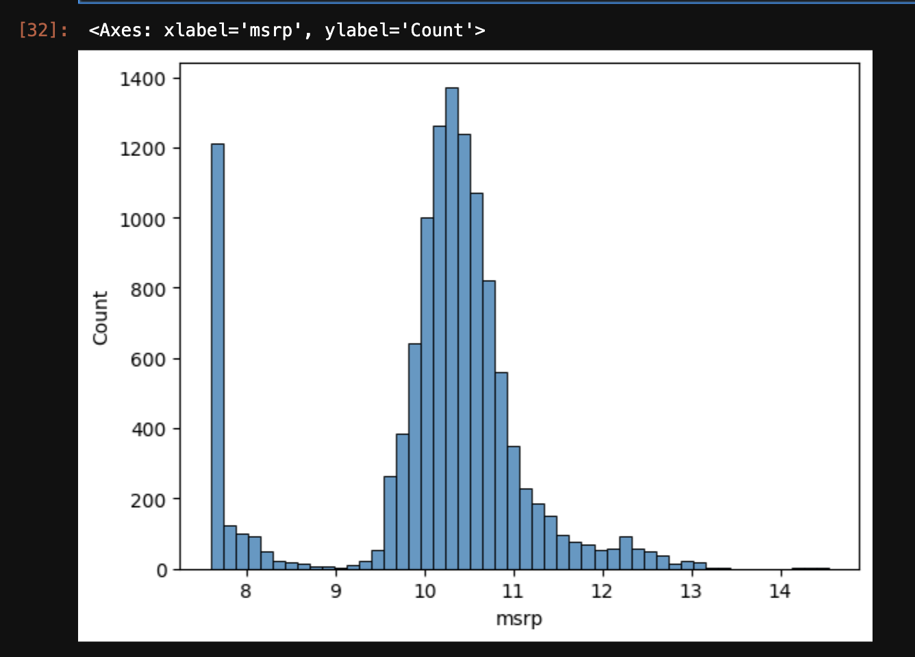
log of 0 gives us a RuntimeWarning for dividing by 0. so, we can instead add 1 to all values, and then take a log. numpy has a built-in way of doing this by using log1p instead - np.log1p([0]) gives array([0.])
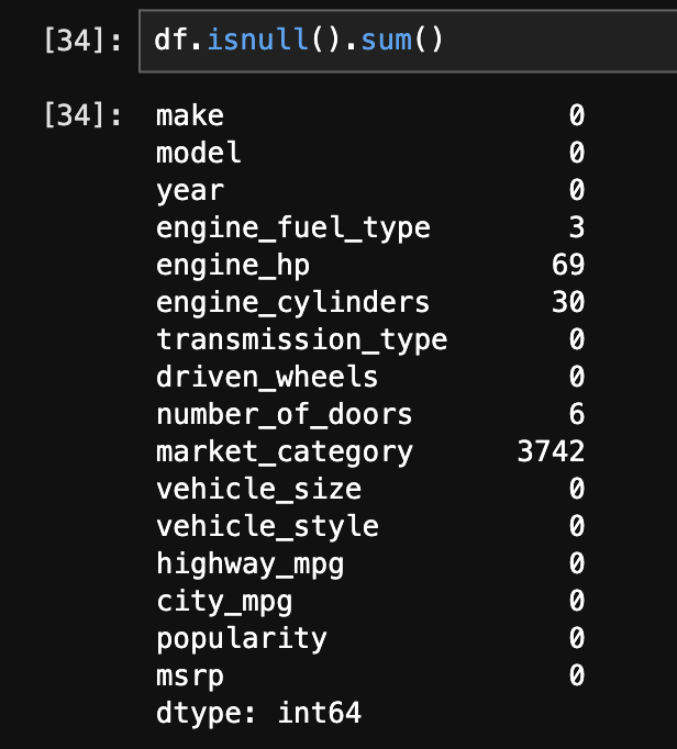
the new histogram now looks as follows - sns.histplot(np.log1p(df['msrp']), bins=50)
next, we get a sense of the missing values in the data using df.isnull().sum()

now, we split the dataset into “training”, “validation”, and “test” sets. first, we determine their lengths -

import math

n = len(df)

n_test = math.floor(0.2 * n)
n_val = math.floor(0.2 * n)
n_train = n - (n_test + n_val)

n_train, n_test, n_val

we observe that our dataset is grouped based on “make”, e.g. all cars with make bmw first and so on

so, if we pick the elements from our dataset serially, e.g. validation first then training, our training data will not have any examples of cars with a make of bmw at all. so, we can instead, use for e.g. the technique below -

idx = np.arange(n)
np.random.shuffle(idx)
idx
# array([6236, 1578,  432, ..., 2381, 7640, 5545], shape=(11914,))

df_train = df.iloc[idx[ : n_train]]
df_test = df.iloc[idx[n_train : n_train + n_test]]
df_val = df.iloc[idx[n_train + n_test : ]]

specify a seed for deterministic results - np.random.seed(2)
finally, the indices of all the datasets would be in random order (since we picked them in random order). so, we can reset the indices again using df_test = df_test.reset_index(drop=True). refer the image below for the before and after -

next, we extract and separate the target variable vector from our feature matrix -

y_train = np.log1p(df_train['msrp'].array)
y_test = np.log1p(df_test['msrp'].array)
y_val = np.log1p(df_val['msrp'].array)
 
del df_train['msrp']
del df_test['msrp']
del df_val['msrp']

the general formula for regression is like this - $g(x_i) = w_0 + x_{i1} \cdot w_1 + x_{i2} \cdot w_2 + … + x_{in} \cdot w_n$
note - $w_0$ is called the “bias term”, which refers to the predictions if we have no information about the car
this can be rewritten as $g(x_i) = w_0 + \sum_{j=1}^{n} x_{ij} \cdot w_j$
assume that $x_{i0} = 1$, then we can rewrite it as $g(x_i) = \sum_{j=0}^{n} x_{ij} \cdot w_j$
so, the idea would probably be to append a column of 1s to the list of features we receive
we know that the summation portion is nothing but essentially a “vector vector multiplication”. so, we can rewrite it again as $g(x_i) = x_i^T \cdot w$
this was for one record (the i in the formula denotes the ith record). when we consider for all the records / training data at once, it basically looks like this ($g(x) = x^T \cdot w$) -
$\begin{pmatrix} 1 & x_{11} & x_{12} & \dots & x_{1n} \\ 1 & x_{21} & x_{22} & \dots & x_{2n} \\ \vdots & \vdots & \vdots & \vdots & \vdots \\ 1 & x_{m1} & x_{m2} & \dots & x_{mn} \end{pmatrix} \cdot \begin{pmatrix} w_0 \\ w_1 \\ w_2 \\ \vdots \\ w_n \end{pmatrix} = \begin{pmatrix} y_1 \\ y_2 \\ \vdots \\ y_m \end{pmatrix}$
we need to calculate “weights” for the actual predictions. we cannot calculate the inverse of the feature matrix, because it is not a “square matrix”, it is (m * (n + 1))
so, we construct a “gram matrix” to make it square. it is defined as $X^T \cdot X$
finally after some basic math, $w$ can be calculated as $(X^T \cdot X)^{-1} \cdot X^T \cdot y$
understand that this calculation would be an “approximation”. this is why the predictions and actual values do not align perfectly for the validation dataset as seen later

some python code for calculating the weights -

def baseline_linear_regression(X, y):
  ones = np.ones(X.shape[0])
  X = np.column_stack([ones, X])

  XTX = X.T.dot(X)
  XTX_inv = np.linalg.inv(XTX)

  w_full = XTX_inv.dot(X.T).dot(y)

  w0 = w_full[0]
  w = w_full[1:]

  return w0, w

now, we extract just the numeric features from the dataframe, since linear regression can only be applied to numerical features -
```
numeric_cols = df_train.dtypes[df.dtypes != 'object'].index
df_train_base = df_train[numeric_cols]
```
next, we need to deal with missing values as otherwise, the matrix and vector multiplication will fail. filling with 0 is like for e.g. “ignoring” a feature. sometimes, it might not make sense. e.g. an engine with missing horsepower might not work, so we might want to fill it with the mean value instead
```
df_train_base = df_train_base.fillna(0)
```
next, we calculate the weights - w0, w = baseline_linear_regression(df_train_base, y_train)
finally, we make the predictions on the validation dataset as follows. note how we first need to perform the same transformations to the validation feature matrix that we did to the training feature matrix -
```
df_val_base = df_val[numeric_cols]
df_val_base = df_val_base.fillna(0)

y_pred = w0 + df_val_base.dot(w)
```
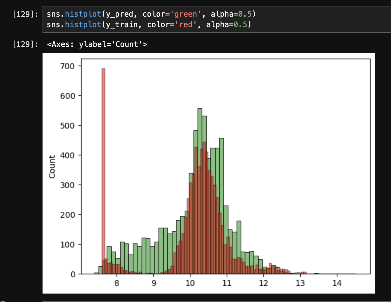
we can compare our predictions with the actual values as follows -
we can evaluate regression models using “rmse” or “root mean square error”. it helps measure the error associated with the model being evaluated. it is the “metric” we discussed in crisp dm it can be used to compare the different models, and then choose the best one. the formula is as follows $\text{RMSE} = \sqrt{\frac{1}{m} \sum_{i=1}^{m} (g(x_i) - y_i)^2}$
here, $g(x_i)$ is the “prediction”, $y_i$ is the “actual value”, and $m$ is the number of records. we can implement it using python as follows -
```
def rmse(y_pred, y):
  e = y_pred - y
  se = e ** 2
  mse = se.mean()
  return math.sqrt(mse)
  
rmse(y_pred, y_val)
# 0.5146325131050283
```
“feature engineering” is the process of creating new features. e.g. we change the year feature to “age” instead
we create a “prepare x” function, so that the different feature matrices like training and validation can simply be passed to it. also notice how we create a copy at the beginning to avoid changing the original dataframe
```
def prepare_features(X):
  numeric_cols = X.dtypes[X.dtypes != 'object'].index
  X = X[numeric_cols].copy()

  X['age'] = X['year'].max() - X['year']
  del X['year']

  X = X.fillna(0)

  return X
```
we see that rmse drops down to 0.49 from 0.51 when we do this
“categorical variables” - typically strings, e.g. make, model, etc. however, some like number of doors are categorical but numbers
we can do analysis on features like this as follows - df_train['number_of_doors'].value_counts()
“one-hot encoding” - we have a binary column for each category value. e.g. the number of doors column is split into - is number of doors 2, is number of doors 3 and so on. each of these hold a 1 or 0, depending on the value that the record has for the number of doors column -
$\begin{pmatrix} 2 \\ 3 \\ 4 \\ 2 \\ \end{pmatrix} = \begin{pmatrix} 1 \\ 0 \\ 0 \\ 1 \\ \end{pmatrix} \begin{pmatrix} 0 \\ 1 \\ 0 \\ 0 \\ \end{pmatrix} \begin{pmatrix} 0 \\ 0 \\ 1 \\ 0 \\ \end{pmatrix}$
as “make” has a lot of unique values, we only take the top 15 values. i guess the unpopular cars with none of the makes would hold a 0 for all the make related categorical columns

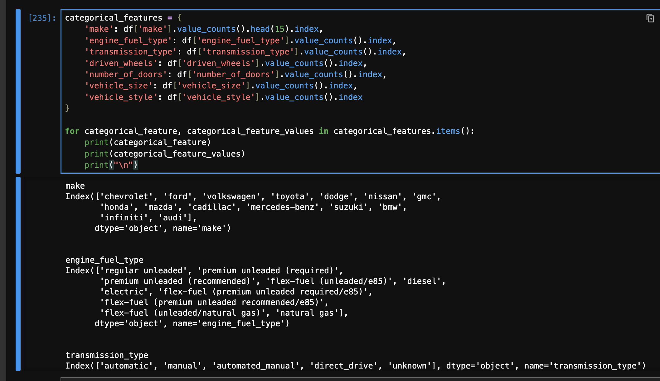
now, we first construct a dictionary as follows -

categorical_features = {
    'make': df['make'].value_counts().head(15).index,
    'engine_fuel_type': df['engine_fuel_type'].value_counts().index,
    'transmission_type': df['transmission_type'].value_counts().index,
    'driven_wheels': df['driven_wheels'].value_counts().index,
    'number_of_doors': df['number_of_doors'].value_counts().index,
    'vehicle_size': df['vehicle_size'].value_counts().index,
    'vehicle_style': df['vehicle_style'].value_counts().index
}

we add this snippet to our prepare_features function -

for feat, vals in categorical_features.items():
    for val in vals:
        X[f'{feat} {val}'] = (X[feat] == val).astype(int)
    del X[feat]

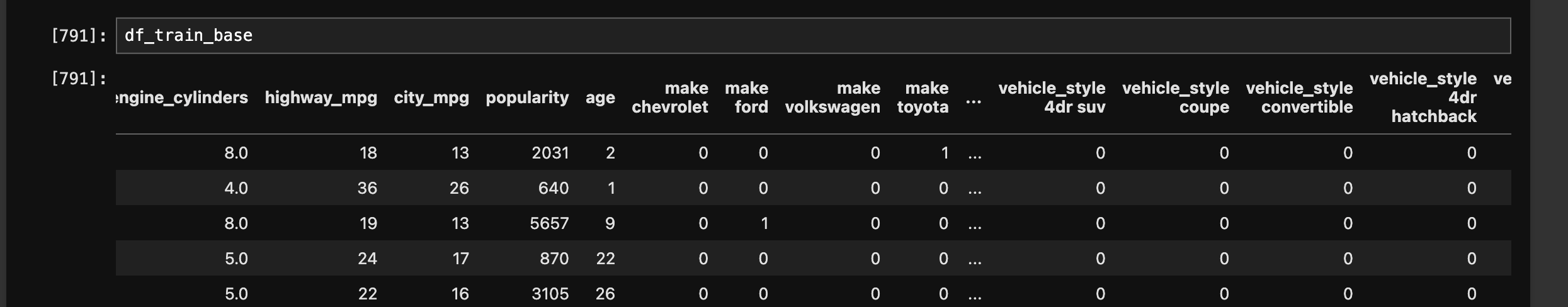
the matrix now looks like this -
however, now when we try predicting, we see the following problems -
- we notice that the rmse is now 1391
- sometimes on rerunning the entire notebook, i see the error that “the matrix is singular”
- w0 / bias shows a very huge value - np.float64(-4129369813575166.5)
- even some of the weights in our vector w are very huge
this happens because the inverse of our “gram matrix” might not exist. we have a lot of features in binary form after we introduced the categorical features. because of this, some of them might become duplicate or basically, some column can be expressed as a linear combination of other columns. when this happens, the inverse of the matrix does not exist. we get the error that “the matrix is singular”. this can be demonstrated using a quick example below, where the second and third columns are identical -
```
x = np.array([
    [1, 2, 2],
    [3, 4, 4],
    [5, 1, 1]   
])

np.linalg.inv(x.T.dot(x))

# LinAlgError: Singular matrix
```
the solution is “regularization”. we add a certain number on the diagonal. this ensures that the columns have different values, and thus can be inverted. this can be done quickly using the identity matrix. the larger the value we add i.e. the larger the multiplier (0.01 below), the more “in control” the weights would be. we can make the following modification to baseline_linear_regression (add the second line) -
```
XTX = X.T.dot(X)
XTX = XTX + (0.01 * np.eye(XTX.shape[0]))
XTX_inv = np.linalg.inv(XTX)
```
note - the regularization technique of adding a value on the diagonal is called “ridge regression”
after this, we see that the rmse becomes 0.44
the regularization value we added i.e. 0.01 is a “hyperparameter”
tuning the model means finding the best possible value of this hyperparameter. so, we change baseline_linear_regression to accept it as a parameter instead, and iterate through its different possible values of the regularization as follows -

one common technique is that after finding the best model, hyper parameters, etc, we again train it but using both the training and validation data together. then, we test it against the testing data -

df_full = pd.concat([df_train, df_test])
df_full.reset_index(drop=True)

y_full = np.concat([y_train, y_val])

df_full_prepared = prepare_features(df_full)
df_test_prepared = prepare_features(df_test)

w0, w = baseline_linear_regression(df_full_prepared, y_full, r)

y_pred = w0 + df_test_prepared.dot(w)
rmse(y_pred, y_test)

finally, recall that the target variable is using log1p, so to get the final price, we use np.expm1

Classification

example - the company determines and sends out discounts and promotions to customers to avoid churning
$g(x_i) = y_i$. we use “binary classification” for the $i$th customer
$y_i$ is the model’s prediction and belongs to {0,1}, where 0 indicates the customer is not likely to churn and 1 indicates the customer is likely to churn
one useful trick to analyze pandas dataframes with lot of columns - df.head().T
data cleanup example for a numerical column -
- when we run df.types, we see totalcharges of type object
- when we try running pd.to_numeric(df.totalcharges), we get the following error - ValueError: Unable to parse string " "
- by some analysis, we can see that there are 11 records with totalcharges as a space
- so, use pd.to_numeric(df.totalcharges, errors='coerce') instead to sets nan for such records

so, our final transformation looks as follows -

df['totalcharges'] = pd.to_numeric(df['totalcharges'], errors='coerce')
df['totalcharges'] = df['totalcharges'].fillna(0)

convert yes / no to integers - df['churn'] = (df['churn'] == 'yes').astype(int)
finally, we run checks for null values using df.isnull().sum()
recall our definition of $y_i$ i.e. churn earlier. so, to get the churn rate of our company, we can calculate the mean of the churn column now - df['churn'].mean()
we will use sckit learn in this section, and not core apis of pandas and numpy directly

splitting the dataset - note how we grab 25% of the full train dataframe so that we have the split of 60-20-20 -

from sklearn.model_selection import train_test_split

full_train_df, test_df = train_test_split(df, test_size=0.2, random_state=1)
train_df, val_df  = train_test_split(full_train_df, test_size=0.25, random_state=1)

  
full_train_df = full_train_df.reset_index(drop=True)
train_df = train_df.reset_index(drop=True)
val_df = val_df.reset_index(drop=True)
test_df = test_df.reset_index(drop=True)

full_train_y = full_train_df['churn'].values
train_y = train_df['churn'].values
val_y = val_df['churn'].values
test_y = test_df['churn'].values

del full_train_df['churn']
del train_df['churn']
del val_df['churn']
del test_df['churn']

now, we try to look at the churns for different “groups”, and compare it to the “global churn” -

df['churn'].mean()
# np.float64(0.2653698707936959)

df.groupby('gender')['churn'].mean()
# gender
# female    0.269209
# male      0.261603

df.groupby('partner')['churn'].mean()
# partner
# no     0.329580
# yes    0.196649

next, we define our numerical and categorical columns -

numerical_columns = ['monthlycharges', 'tenure', 'totalcharges']
categorical_columns = ['contract', 'dependents', 'deviceprotection', ... , 'techsupport']

and we ensure we only use them for our analysis. we do not want to have columns like “customer id”, which are not relevant features for our analysis -

full_train_df = full_train_df[categorical_columns + numerical_columns]
train_df = train_df[categorical_columns + numerical_columns]
val_df = val_df[categorical_columns + numerical_columns]
test_df = test_df[categorical_columns + numerical_columns]

observe the unique values per category - df[categorical_columns].nunique()

contract            3
dependents          2
deviceprotection    3
gender              2
...

intuition - it tells us that the gender does not play a significant role in churn, while having a partner does
technique 1 - “churn rates” - calculated as (churn of a group) - (global churn rate). if it is > 0, it means that the group is at a higher risk of churning. however, as we saw above, the “magnitude” matters as well i.e. customers having no partners are at a much higher risk of churning than the customer being a female
technique 2 - “risk ratios” - calculated as (churn rate of group) / (global churn rate). a risk ratio > 1 indicates a higher risk of churning, while a risk ratio < 1 indicates a lower risk

so, we can perform some “exploratory data analysis” for all the categorical variables as follows -

from IPython.display import display
  
for categorical_column in categorical_columns:
  display(df.groupby(categorical_column)['churn'].mean())
  print()

“mutual information” - a concept from “information theory”, that tells us how much we can learn about one random variable, if we know about another random variable
example how much do we learn about “churn”, if we know about a certain feature, e.g. type of contract - “month-to-month” vs “one year” vs “two year”
sckit learn already implements this for us, and we can use it as follows. note - the order of columns does not matter. it clearly shows how gender does not matter unlike type of contract -
```
from sklearn.metrics import mutual_info_score

mutual_info_score(df['churn'], df['contract']) # 0.09845305342598942
mutual_info_score(df['churn'], df['gender']) # 3.7082914405128786e-05
```
note - “mutual information” is applicable for “categorical variables” only
so, we can use df.apply to get the mutual information score for all the columns. apply accepts a function that gets called for every column of the dataframe. we also sort it in decreasing order to quickly analyze which columns are important -
```
df[categorical_columns].apply(lambda series: mutual_info_score(series, df['churn'])).sort_values(ascending=False)

# contract            0.098453
# onlinesecurity      0.064677
# techsupport         0.063021
# ...
```
for numerical variables, we use “correlation”. also called “pearson’s correlation”
it is denoted by $r$, and $r \in [-1, 1]$
negative correlation indicates that as for e.g. value of one variable increases, the other variable tends to decrease and vice versa
the higher the magnitude, the more they are correlated - upto 0.2 is “low correlation”, 0.2 - 0.5 is “moderate correlation” and otherwise it is “strong correlation”
look at the correlation of numerical features - df[numerical_columns].corrwith(df['churn'])
here, we see a negative correlation with tenure - which basically means the longer a person stays with the company, the lesser is the churn rate. we can further perform analysis as follows, e.g. compare the churn rate for people who have stayed less than vs more than a year
```
df[df['tenure'] <= 12]['churn'].mean() # np.float64(0.47438243366880145)
df[df['tenure'] > 12]['churn'].mean() # np.float64(0.17129915585752523)
```
this time, we perform one hot encoding using scikit learn -
```
from sklearn.feature_extraction import DictVectorizer
```

since we are using “dict vectorizer”, we use .to_dict(orient='records') to convert the dataframe to a list of dictionaries

train_dicts = train_df.to_dict(orient='records')
# [
#   {'customerid': '8015-ihcgw', 'gender': 'female', ... 'totalcharges': 8425.15},
#   {'customerid': '1960-uycnn', 'gender': 'male', .. 'streamingmovies': 'no'},
# ...

we need to kind of “train” the vectorizer on some sample data. using that sample data, the vectorizer determines the different categories and their values, and accoridngly decide on the columns etc. note - we might end up having a lot of zeroes, and scikit learn would use compressed sparse matrices for efficiency etc. however, we set sparse as false here to have the original one hot encoding behavior of 0 / 1 for each value of the category as we saw in regression
```
dv = DictVectorizer(sparse=False)
dv.fit(train_dicts)
```
note how we specified passed in all columns i.e. numerical and categorical to the fit. it is intelligent enough to leavre the numerical columns untouched, e.g. senior citizen and total charges would become - [senior citizen=0, senior citizen=1, total charges]
why is this important - because remmeber, while we do not encode the numerical columns in this step, they still have weights in our actual prediction (how logistic regression works is discussed later)

finally, we obtain the matrices with the encoding using transform

train_mat = dv.transform(train_dicts)
  
# array([[0.00000e+00, 1.00000e+00, 0.00000e+00, ..., 1.00000e+00,
#       4.10000e+01, 3.32075e+03],
#      [0.00000e+00, 0.00000e+00, 1.00000e+00, ..., 0.00000e+00,
#       6.60000e+01, 6.47185e+03],

note how it is no longer a dataframe, but a 2d numpy array i guess? we can obtain the corresponding feature names for the 2d array as follows -

dv.get_feature_names_out()

# array(['contract=month-to-month', 'contract=one year', 'contract=two year', 
#  'dependents=no', 'dependents=yes',

so, the final code snippet is as follows -

dv = DictVectorizer(sparse=False)

train_dicts = train_df.to_dict(orient='records')
val_dicts = val_df.to_dict(orient='records')

dv.fit(train_dicts)

train_mat = dv.transform(train_dicts)
val_mat = dv.transform(val_dicts)

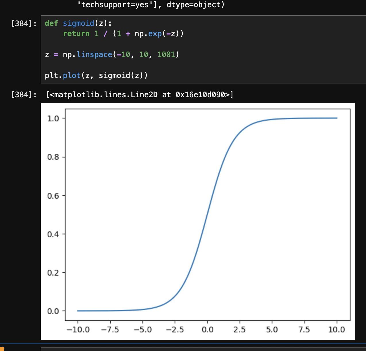
recall how in our case, $x \in [-\infty, \infty]$ (i.e. x can be any real number, e.g. tenure), while $y \in {0, 1}$ (i.e. y can only be 0 or 1 i.e. the churn). in case of “logistic regression”, we apply the “sigmoid” function to the “linear regression” formula. the linear regression formula can give us any value from $-\infty$ to $+\infty$, while the sigmoid function converts the output to be between 0 and 1, thus helping us with “binary classification”. at $-\infty$, its output is 0 and at $+\infty$, its output is 1. at 0, its output is 0.5
formula of sigmoid - $\sigma(z) = \frac{1}{1 + e^{-z}}$
we can look at its graph as follows -

so, we can use the logistic regression model as follows -

from sklearn.linear_model import LogisticRegression
  
model = LogisticRegression()
model.fit(train_mat, train_y)

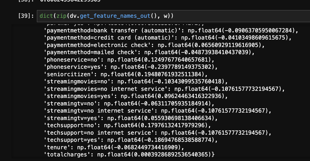
we can obtain the weights from the model like this
```
w = model.coef_[0]
w0 = model.intercept_[0]
```
understand what the weights are - they are the coefficients for all the features we have. e.g. look at the below image on how we can easily look at the correlation of each feature with the target variable. also, notice how numerical columns like total charges were considered automatically, as the dict vectorizer did not touch them -
we can use the model as follows. the first one is called “hard predictions”, as it would have the exact label of 0 or 1 (churn or not churn). the second one is called “soft predictions”, as it would give the probabilities instead. note how in case of soft predictions, we see two elements per record as the first one is probability of 0 (not churn), and second is probability of 1 (churn)
```
model.predict(val_mat) # array([0, 0, 0, ..., 0, 1, 1], shape=(1409,))
model.predict_proba(val_mat) # array([[0.98157471, 0.01842529], ..., [0.30467382, 0.69532618]], shape=(1409, 2))
```
recall that we used rmse in regression to measure the accuracy of our model. in this case we use a method called “accuracy” as follows i.e. average number of times our predictions were correct -
```
val_y_predict = model.predict(val_mat)
(val_y_predict == val_y).astype('int').mean()
```

we can also use scikit learn for the same -

from sklearn.metrics import accuracy_score

accuracy_score(val_y, model.predict(val_mat))

finally, we do it for the training and validation dataset together, and predict it against the test dataset -

full_train_dicts = full_train_df.to_dict(orient='records')
test_dicts = test_df.to_dict(orient='records')

dv = DictVectorizer(sparse=False)

dv.fit(full_train_dicts)

full_train_mat = dv.transform(full_train_dicts)
test_mat = dv.transform(test_dicts)

model = LogisticRegression()
model.fit(full_train_mat, full_train_y)

pred_y = model.predict(test_mat)

accuracy_score(test_y, pred_y)

Evaluation

“accuracy” as we saw in classification is the number of correct predictions / total number of predictions
how the prediction was working - we used regression that spit out a real number, which was then passed via the sigmoid function to clamp it between 0 and 1. finally we used a threshold of 0.5 to label it as 0 or 1 i.e. below 0.5 is 0 (not churn) and above 0.5 is 1 (churn). this 0.5 is called the “decision threshold”. below is a python code breakdown. recall how predict_proba works from classification i.e. using soft predictions. so, we only select its second column i.e. the probability of churn, and then look at all its values where it is >= 0.5
```
pred_y_proba = model.predict_proba(test_mat)[:,1]
accuracy_score(test_y, pred_y_proba >= 0.5)
```
my understanding - the decision threshold is therefore like a hyperparameter, which we can test as follows, and we see that accuracy is a little higher at for e.g. 0.6 -
using decision threshold of 1 basically means we say no customers are going to churn. however, we can see that even this dummy model has accuracy of 75%, while our decision threshold of 0.5 has 81% accuracy
this is happening because the data is “unbalanced”. this is called “class imbalance”, as we have more instances of 1 category than the other. 75% of the testing dataset contains of people who are non churning -
```
(test_y == 1).sum(), (test_y == 0).sum()
# (np.int64(348), np.int64(1061))
```
so, instead of using “accuracy”, we use “confusion table”
we have four scenarios. true means our prediction was correct, positive means that our prediction belongs to the “positive class” / 1 / customer actually churned
- “true positive” - we predicted churn, customer churned. $g(x_i) >= t$, $y_i = 1$
- “true negative” - we predicted no churn, customer did not churn. $g(x_i) < t$, $y_i = 0$
- “false positive” - we predicted churn, customer did not churn. $g(x_i) >= t$, $y_i = 0$
- “false negative” - we predicted no churn, customer churned. $g(x_i) < t$, $y_i = 1$

we can write it in python code as follows -

actual_positive = (test_y == 1)
actual_negative = (test_y == 0)
  
t = 0.5
predict_positive = (pred_y_proba >= t)
predict_negative = (pred_y_proba < t)
  
tp = (predict_positive & actual_positive).sum()
tn = (predict_negative & actual_negative).sum()
fp = (predict_positive & actual_negative).sum()
fn = (predict_negative & actual_positive).sum()
  
tp, tn, fp, fn
# (np.int64(204), np.int64(943), np.int64(118), np.int64(144))

this “confusion matrix” is usually represented in the following manner. we then “normalize” it / see the percentages of each type -

confusion_matrix = np.array([
  [tn, fp],
  [fn, tp]
])
confusion_matrix / confusion_matrix.sum()

# array([[943, 118], [144, 204]])
# array([[0.66926899, 0.08374734], [0.10220014, 0.14478353]])

based on the confusion matrix, we can also see that “accuracy” was basically (tp + tn) / (tp + tn + fp + fn)
“precision” - fraction of correct positive predictions. it can be calculated as (tp / (tp + fp)). e.g. in our case, it would mean that we would send the promotional email to an extra 33% of people who should not have gotten the email, thus leading to potential losses
```
p = tp / (tp + fp)
p # np.float64(0.6335403726708074)
```
“recall” - fraction of actual positives that were correctly predicted. it can be calculated as (tp / (tp + fn)). e.g. in our case, it would mean that we would correctly send the email to only 58% of the customers who would actually churn, thus missing out on the remaining customers
```
r = tp / (tp + fn)
r # np.float64(0.5862068965517241)
```
so, while the accuracy was high, precision and recall are not. hence, accuracy can be misleading in case of for e.g. “class imbalance”
now, we will explore “roc curves” i.e. “receiver operating characteristics”
it is a method of evaluating the performance of a binary classification model across many “thresholds” at once
we are interested in two values fpr and tpr
“fpr” or “false positive rate” = (fp / (fp + tn)) - basically, 1st row of confusion matrix i.e. where target variable is 0
“tpr” or “true positive rate” = (tp / (tp + fn)) - basically, 2nd row of confusion matrix i.e. where target variable is 1
note - looks like tpr and recall have the same formula?
the goal is to minimize false positive rate / maximize true positive rate
roc curves looks at multiple thresholds at once
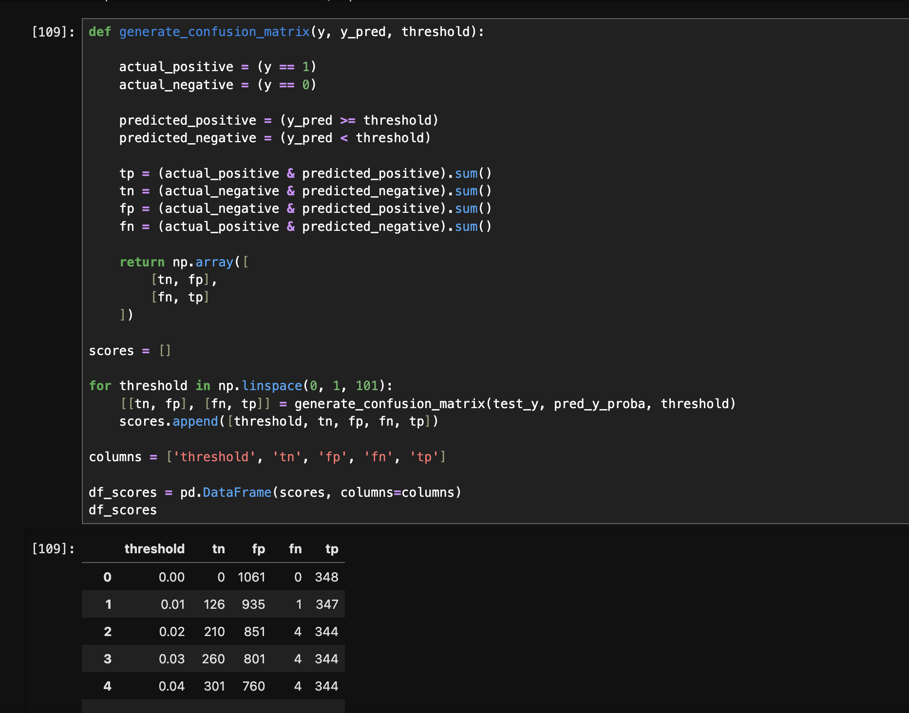
first, we generate the following dataframe for the different thresholds and their respective values for the confusion matrix -

next, we compute the remaining columns as follows -

df_scores['precision'] = df['tp'] / (df['tp'] + df['fp'])
df_scores['recall'] = df['tp'] / (df['tp'] + df['fn'])

df_scores['fpr'] = df['fp'] / (df['fp'] + df['tn'])
df_scores['tpr'] = df['tp'] / (df['tp'] + df['fn'])

df_scores

note - whatever we did manually till now, can be done automatically using scikit learn as follows. we just pass it the actual y and probabilities, and it returns us all three - fpr, tpr and thresholds -
```
from sklearn.metrics import roc_curve
  
fpr, tpr, thresholds = roc_curve(test_y, pred_y_proba)
```

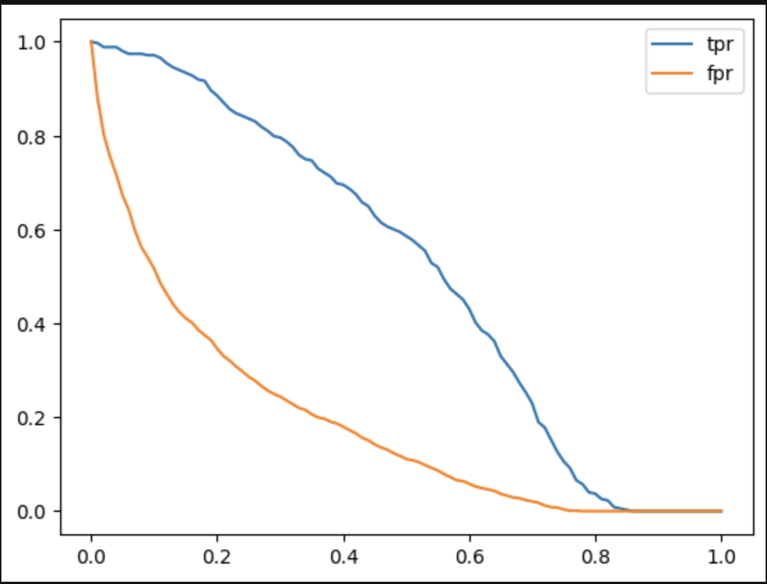
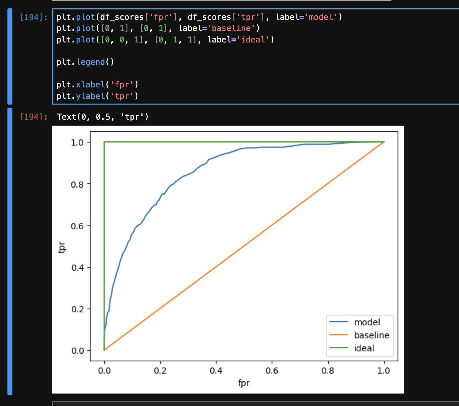
next, we can plot the roc curves as follows -

plt.plot(df_scores['threshold'], df_scores['tpr'], label='tpr')
plt.plot(df_scores['threshold'], df_scores['fpr'], label='fpr')
plt.legend()

we want fpr to be towards 0, and tpr to be towards 1
now, we now plot tpr and fpr against each other. we plot the following three graphs
note - below is intuition, there may be more math to it
at the beginning of the curves, threshold is basically 0. so, our model does not predict anything as positive. so, fpr and tpr are both typically 0
at the end of the curves, our threshold is 1. so, our model does not predict anything as negative. hence, we have both tpr and fpr as 1
first, we add a baseline. the idea is usually that a models should never go below the baseline. the line for this is a straight line. this means as our tpr increases (which is good), our fpr increases as well (which is bad)
```
plt.plot([0, 1], [0, 1], label='baseline')
```
then, we also plot our model’s tpr and fpr
finally, we plot our “north star” / ideal state, which is basically tpr = 1 and fpr = 0. to complete the curve, we add the two additional points for thresholds 0 and 1
```
plt.plot([0, 0, 1], [0, 1, 1], label='ideal')
```
“area under roc curve” is a useful metric of calculating the performance of a binary classification model
for the ideal model, the area under the roc curve is 1, while for the baseline model, the area under the curve is 0.5. so, the area under roc curve for our model should be somewhere between 0.5 and 1

scikit learn has a function called “auc” to calculate the area under any curve. we can use it as follows (recall that fpr and tpr were already calculated using roc_curve) -

from sklearn.metrics import auc

print(auc(fpr, tpr)) # model - 0.8569948649614871
print(auc([0, 0, 1], [0, 1, 1])) # ideal - 1.0
print(auc([0, 1], [0, 1])) # baseline - 0.5

intrerpretation of area under roc curve - the probability that a randomly selected positive instance is ranked higher than a randomly selected negative instance. ranked higher is basically means higher probability. instance basically means actual labels / test y. this happens because assume we predict probability as 0.3. say our threshold is 0.5, we classify it as not churning, but it might actually be a positive instance i.e. a churned customer. so, area under roc curve basically tells us the probability that a randomly selected churning customer actually has higher probability as per our model than a randomly selected non churning customer. see how we can write the following python code to get the same result as the auc above -
```
import random

trials = 1000000

neg_instances = pred_y_proba[test_y == 0]
pos_instances = pred_y_proba[test_y == 1]

success_count = 0

for i in range(trials):
  probab_neg = random.choice(neg_instances)
  probab_pos = random.choice(pos_instances)

  success_count += (probab_pos > probab_neg)

success_count / trials # np.float64(0.857021)
```

Cross Validation

“cross validation” is applied during the “parameter tuning step”, where we select the best parameters
e.g. LogisticRegression that we used in classification accepts a parameter C, similar to the regularization parameter we discussed
the full training dataset (i.e. training + validation dataset) is split into k “folds”. we train the model on k-1 folds and validate it on the remaining fold. this process is repeated k times, with each fold being used as the validation set once. e.g. train on 1,2 and validate on 3, train of 1,3 and validate on 2 and finally train on 2,3 and validate on 1
we keep computing the auc for the remaining fold, and we finally compute the mean and standard deviations across all these k folds
we can do this using scikit learn using “kfold”. we construct it by specifying the no. of folds, the shuffle decision and a seed
```
from sklearn.model_selection import KFold

kfold = KFold(n_splits=3, shuffle=True, random_state=1)
```

its split method returns us a generator which we can iterate over as follows

scores = []

for train_idx, val_idx in kfold.split(full_train_df):
  train_df = full_train_df.iloc[train_idx]
  val_df = full_train_df.iloc[val_idx]
  # ...
  scores.append(auroc)

finally, we can compute the stats as np.mean(scores) and np.std(scores)
use case for “cross validation” - the general method is called “holdout dataset”, and it works when we have a large dataset. we use cross validation when our dataset is small / we want to know the standard deviation of our model across different folds

Deployment

using “model deployment”, we can reuse the model without retraining / rerunning the code
we deploy the model as a web service so that external services like marketing service can send requests to the server to get predictions
first, we train and save the model, e.g. using pickle. note how we save the dictionary vectorizer as well -
```
import pickle

with open('model.bin', 'wb') as file:
  pickle.dump((dv, model), file)
```
when doing this, we can add hyper parameters to the file name to easily differentiate between the different model versions
now, we first create a dummy customer object as follows. we load it from the test df itself for now -
```
customer = test_df.iloc[0]
customer.to_dict()
```

now, we can load and use our saved model as follows -

# we get a customer. we load it from test df for now
# { 'contract': 'one year', 'dependents': 'no', ... 'tenure': 41, 'totalcharges': 3320.75 }

import pickle

with open('model.bin', 'rb') as file:
  dv, model = pickle.load(file)

# transform accepts an array, so we wrap it around one
customer_mat = dv.transform([customer])
model.predict_proba(customer_mat)
# array([[0.93249759, 0.06750241]])

below example uses flask to create api endpoints for the predictions -

import pickle
from flask import Flask, request, jsonify

app = Flask('predict')

with open('model.bin', 'rb') as file:
  dv, model = pickle.load(file)

@app.route('/predict', methods=['POST'])
def predict():
  customer = request.get_json()

  customer_mat = dv.transform([customer])
  probability = model.predict_proba(customer_mat)[0][1]

  return jsonify({
      "probability": probability
  })

app.run(debug=True, host='0.0.0.0', port=8080)

now, we can make predictions via for e.g. postman -

Decision Trees

we build a credit risk scoring model, that predicts whether a bank should lend money to a client or not
we analyze historical data of customers who defaulted, given the details like the amount they borrowed, their age, marital status, etc
this is a “binary classification” problem, where the model returns a 0 (the client is likely to payback the loan, and the bank will approve the loan) or 1 (the client is likely to default, and the bank will not approve the loan)
first, we perform some data preparation
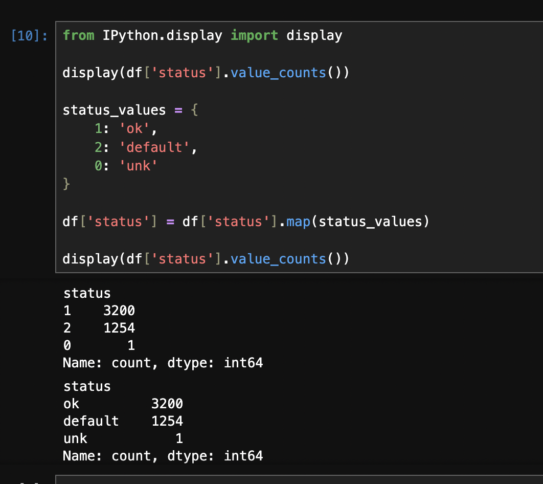
we can use the following code to map numbers to strings for categorical features. i am guessing this is needed because it is for e.g. used by dict vectorizer. look at the before vs after of value_counts -
```
status_values = {
    1: 'ok',
    2: 'default',
    0: 'unk'
}

df['status'] = df['status'].map(status_values)
```
some columns have 99999999 for missing values. we can confirm this by running df.describe(), as it shows the various stats of numerical columns. we can fix it as follows. after making this fix, we see how the various statistics like mean etc for these columns start making sense as well -
```
df['income'] = df['income'].replace(99999999, np.nan)
```
we can also fill them with 0s instead based on our judgement
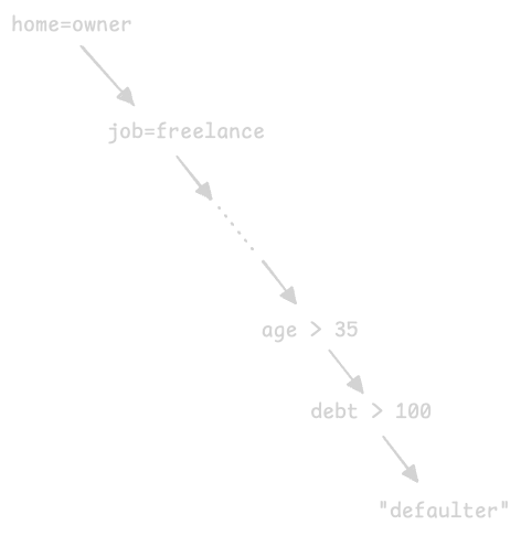
“decision trees” - it has “nodes” which represent conditions (e.g. customer has assets with value > 5000), and the “branches”, which represent true or false. the records go through this tree from the root, until they reach the terminal node called “leaves”, which contain the value of the target variable
these rules are learnt from the data - e.g if the customer has no past records of borrowing, and if they have no house, then they are a defaulter

using a decision tree classifier from scikit learn -

from sklearn.feature_extraction import DictVectorizer
from sklearn.metrics import roc_auc_score

dv = DictVectorizer(sparse=False)
dv.fit(train_dicts)

train_mat = dv.transform(train_dicts)
dtc = DecisionTreeClassifier()
dtc.fit(train_mat, train_y)

val_mat = dv.transform(val_dicts)
val_proba_y = dtc.predict_proba(val_mat)[:,1]
roc_auc_score(val_y, val_proba_y) # 0.654

train_proba_y = dtc.predict_proba(train_mat)[:,1]
roc_auc_score(train_y, train_proba_y) # 1.0

so, 1 common problem with decision trees we see above - “overfitting”. we can see that auc for roc is 1 for the training dataset, but around 65% for the validation dataset. this is happening because our decision trees grow to large depths, thus memorizing the training data and failing when given the testing data. the leaf nodes then end up containing only 1 or 2 training data records

so, we limit the depth of the tree, and we see that the scores improve automatically -

dtc = DecisionTreeClassifier(max_depth=3)

roc_auc_score(val_y, val_proba_y) # 0.7389079944782155
roc_auc_score(train_y, train_proba_y) # 0.7761016984958594

we can visualize the decision tree as follows -

from sklearn.tree import export_text

print(export_text(dtc, feature_names=dv.get_feature_names_out()))

# |--- records=no <= 0.50
# |   |--- seniority <= 6.50
# |   |   |--- amount <= 862.50
# |   |   |   |--- seniority <= 0.50
# |   |   |   |   |--- class: 1
# |   |   |   |--- seniority >  0.50
# |   |   |   |   |--- class: 0
# |   |   |--- amount >  862.50
# |   |   |   |--- assets <= 8250.00
# |   |   |   |   |--- class: 1
# |   |   |   |--- assets >  8250.00
# |   |   |   |   |--- class: 0
# |   |--- seniority >  6.50
# |   |   |--- income <= 103.50
# |   |   |   |--- assets <= 4500.00
# |   |   |   |   |--- class: 1
# |   |   |   |--- assets >  4500.00

how a decision tree learns - using “missclassification”. assume we have a condition for customers having assets > 3000 on the root node of the decision tree. this would split our data into two parts. however, the left part can have both defaulters and non-defaulters, and so can the right part

left_non_defaulters = (df[df['assets'] > 3000]['status'] == 'ok').sum() # 1776
left_defaulters = (df[df['assets'] > 3000]['status'] == 'default').sum() # 419

right_non_defaulters = (df[df['assets'] <= 3000]['status'] == 'ok').sum() # 1397
right_defaulters = (df[df['assets'] <= 3000]['status'] == 'default').sum() # 815

so, “missclassification rate” for right part basically means, assume our model would have predicted “defaulter” for right part. what is the rate by which it would have failed? it would be 1397 / (815 + 1397) = 0.368 in this case
then, say we can say take weighted average of left and right parts (weighted because for instance, no. of records on left can be more than right)
we are basically trying to evaluate the “impurity” at the leaf nodes
“missclassification” is a type of this impurity check for decision trees. however, we can use other metrics as well, e.g. “entropy” and “gini”
“threshold” - while we hardcoded 3000, we would have to iterate for different possible values of this threshold, to “minimize the impurity”

the pseudo algorithm for how decision trees work can be as follows (recall how we hardcoded a threshold of 3000, but that too can change) -

for all feature in features:
  for all threshold in thresholds for feature:
    split the dataset using feature > threshold
    compute the impurity (e.g. missclassification rate) for the left and right parts
    compute score using weighted average of the two halves

select the best (feature + threshold) combination with the lowest impurity
use it to split the dataset into left and right

now, we keep applying this algorithm recursively to the left and right subtrees of our nodes
the stopping criteria for this recursion can be -
- when the group is already pure / has reached a certain level of purity
- when the tree reaches the depth (we explored this earlier for overfitting)
- when the group size becomes too small to split into left and right. e.g. if we have 100 samples, it makes sense to run the algorithm, but it does not when the group size is say 5

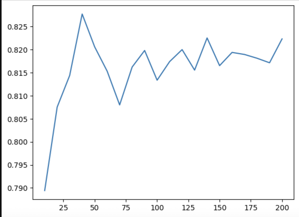
so, we can now tune our model using the three parameters - “max depth” and “min samples leaf” (i.e. a node would be split only if it contains at least these many records)

for max_depth in [1, 2, 3, 4, 5, 6]:
  for min_samples_leaf in [1, 2, 5, 10, 15, 20, 25, 30, 35, 40, 45, 50]:

    dtc = DecisionTreeClassifier(max_depth=max_depth, min_samples_leaf=min_samples_leaf)
    dtc.fit(train_mat, train_y)

    val_proba_y = dtc.predict_proba(val_mat)[:,1]
    score = roc_auc_score(val_y, val_proba_y)

    print("%2d, %3d: %.3f" % (max_depth, min_samples_leaf, score))

one technique in case of large datasets - to avoid the m*n loop, we first try finding the optimal subset of max depths first by setting a hard value for min sample leaf. then, we try finding the optimal value for min sample leaf using this subset of max depths that we obtained
the lesser the depth of the tree, the more it tends to overfit
note - while we only use it for classification here, decision trees can be used for regression as well

Random Forest

“ensemble learning” - multiple models called “weak learners” are combined to solve a particular problem
“random forest” - an example of ensemble learning where each model is a decision tree
the idea is that each decision tree gets a different subset of features. e.g. we have 10 features, the first decision tree gets trained on 7 features, the second on a different set of 7 features, and so on

then, we compute the average using the probabilities from all the decision trees. the code for it is as follows -

from sklearn.ensemble import RandomForestClassifier

rfc = RandomForestClassifier(n_estimators=10)
rfc.fit(train_mat, train_y)

val_proba_y = rfc.predict_proba(val_mat)[:,1]
roc_auc_score(val_y, val_proba_y)

note the use of “random state”. this is for the random subset of features assigned to the different decision trees

so apart from depth and min samples in leaf nodes, we have a third hyperparameter called “no. of estimators” that we can tune as well (i.e. no. of decision trees used in random forest)

scores = []

no_of_trees_list = list(range(10, 201, 10))

for no_of_trees in no_of_trees_list:
    rfc = RandomForestClassifier(n_estimators=no_of_trees)
    rfc.fit(train_mat, train_y)
    val_proba_y = rfc.predict_proba(val_mat)[:,1]
    score = roc_auc_score(val_y, val_proba_y)
    scores.append(score)

plt.plot(no_of_trees_list, scores)

we can see how it peaks at around 40 decision trees -
random forest makes use of “bootstrapping”. in bootstrapping, different subsets of data is created using “sampling with replacement”. “sampling” means picking randomly, while “with replacement” means we might end up having duplicates / missing values in a particular bootstrap sample. my understanding - say our dataset is (a, b, c, d, e). three different bootstrap samples created can be (a, a, c, d, b), (b, e, e, c, a), (d, a, e, b, c). see how each bootstrap sample can have some duplicates and some missing data points. now, each of the three decision trees get trained using a different bootstrap sample, thus making the model more “robust”, less likely to overfit, etc
so, the word “random” in random forest is for two things - this bootstrapping approach, and the random subset of features used by each decision tree

Gradient Boosting

we create a model based on the dataset
we look at the errors, and create a new model to correct these errors
we repeat this process, and keep adding new models to the “ensemble”
unlike random forrest where each model trains independently / in parallel, the models here are trained sequentially, by improving on the errors made by the previous model

xgboost can help implement this technique efficiently. first, we created the matrices used by xgboost. note how we leverage scikit learn’s dict vectorizer outputs here -

import xgboost as xgb

features = list(dv.get_feature_names_out())

train_d = xgb.DMatrix(train_mat, label=y_train, feature_names=features)
val_d = xgb.DMatrix(val_mat, label=y_val, feature_names=features)

then, we train the model as follows -


xgb_params = {
    'eta': 0.3,
    'max_depth': 1,
    'min_child_weight': 1,

    'objective': 'binary:logistic',
    'nthread': 8,

    'seed': 1,
    'verbosity': 1
}

model = xgb.train(xgb_params, train_d, num_boost_round=200)

# .8328207115352014

“max_depth” and “min_child_weight” is similar to “max depth” and “min samples leaf” of scikit learn
“num_boost_round” specifies how many times the improvement process happens. we can log the improvement in each subsequent model after each step as follows -
```
watch_list = [(train_d, 'train'), (val_d, 'val')]
xgb.train(xgb_params, train_d, evals=watch_list, num_boost_round=200)
```
now, we will see the loss after each training step as follows -
“eta” - this is the “learning rate”. it indicates how fast the model learns. recall how in gradient boosting we incrementally improve the models. learning rate determines the weights we use for the features in the current improved model to improve the predictions. e.g. if we use 0.01, it learns very slowly, and we need to increase the number of boosting rounds for the model to finish learning
one technique of finding the hyperparameters - first, find the best value of “eta”, then “max depth” and finally “min child weight”
conclusion - xgboost models tend to have better performances for tabular data (i.e. dataframes with features). however, they need more care when finetuning hyperparameters, else they tend to overfit

MLOps Introduction

mlops - set of best practices to put machine learning into production
problem - predicting the duration of a taxi trip
“mlops maturity” has the following levels
level 0 - we use jupyter notebooks, and there is no automation
level 1 - we have devops but no mlops. our system has the best practices of software engineering - ci cd, automated releases, operational metrics (e.g. requests per second), unit and integration tests. however, it is not machine learning aware i.e. it does not have any special support for machine learning workflows
level 2 - we have a “training pipeline” (an automated script to train the model), “experiment tracking” and “model registry” in place
level 3 - “automated deployment” - we can easily deploy models with very low friction. it supports features like “a/b testing”. additionally, we have “monitoring” in place
level 4 - when there is a drop in the performance of our models, our “monitoring” systems catch this drift automatically, and then automatically run the “training pipeline” and “deploy” the new model automatically. we can do the same thing for functionalities like a/b testing

Experiment Tracking

“experiment tracking” - the process of keeping track of all the information for an experiment, like code, environment, the ml model, its different hyper parameters, metrics, etc
an “experiment” is the entire process where data scientists come up with the ml models, while an “experiment run” is each trial of the different hyper parameters etc that the data scientist may make
advantages of experiment tracking - reproducibility, collaboration in organizations, etc
the earlier methods involved using spreadsheets, mentioning the hyper parameters and tracking metrics like true positives, accuracy, etc in the different columns. issues - prone to human error, not as effective for collaboration, etc
“mlflow” - an opensource platform for managing the entire ml lifecycle
with each run, we keep track of multiple things described below -
- “parameters” - not only hyper parameters, but also include things like path of dataset etc
- “metrics” - metrics like accuracy from training / validation / test dataset
- “metadata” - e.g. “tags” to filter runs easily
- “artifacts” - any file, e.g. visualizations
- “model” - we can also log the model itself as part of experiment tracking
- code, commit sha, start and end times, author name, etc
mlflow is just a python package. run uv add mlflow and then mlflow ui to access it at http://localhost:5000
my understanding - two things are needed for the complete setup of mlflow in a production environment - an object storage (e.g. s3) for storing artifacts and a database (e.g. postgres) used by model registry
we set it up as follows - set experiment creates a new experiment if none exist, and it appends all future runs to this experiment
```
import mlflow
  
mlflow.set_tracking_uri("http://localhost:5000")
mlflow.set_experiment("tripdata")
```

creating a run for the experiment can be done as follows, post which we can browse through the ui -

with mlflow.start_run():

  alpha = 0.01
  mlflow.log_param("alpha", alpha)
  lasso = Lasso(alpha)

  lasso.fit(train_X, train_y)

  pred_y = lasso.predict(val_X)

  rmse = root_mean_squared_error(val_y, pred_y)
  mlflow.log_metric("rmse", rmse)
  print(rmse)

however, even this part can be automated using “auto log”. find the list of supported libraries here. notice how we just wrapped it around “start run”, and all the parameters and metrics were logged automatically
```
mlflow.autolog()
# ...
with mlflow.start_run():

  lr = LinearRegression()
  lr.fit(train_X, train_y)

  pred_y = lr.predict(val_X)

  rmse = root_mean_squared_error(val_y, pred_y)
  print(rmse)
```
what we can do is tag the runs of all models and their combinations of hyper parameters using the same set of tags. this way, we can easily compare the metrics of all these runs using different kinds of visualizations like scatter plots etc
note - when choosing the model, do not just pick the model with the best metrics. such a model might be complex, e.g. decision trees might have lot of depth. so, pick the best model based on your judgement
just like we used spreadsheets for experiment tracking earlier, we could use different file names and a custom folder structure for tracking different models and their versions. however, there is manual effort involved here, and it does not tell us the hyper parameters we used for coming up with the model etc
mlflow makes this much easier, by providing us with a “model management” solution
on going to /experiments/<experiment-id>/models, we can see the different models being added automatically due to auto logging. otherwise, we can also use mlflow.log_model if we would like to do this manually. it will also save the dependency requirements using conda.yaml, requirements.txt, etc automatically. i saw that a generic name called “models” was being used for all models. i used this approach to customize the name -
```
mlflow.autolog(log_models=False)
# ...
with mlflow.start_run():
  lr = LinearRegression()
  # ...
  mlflow.sklearn.log_model(sk_model=lr, name="lr_trip_data")
```
however, we might still have to add some things manually. e.g. we might want to use log_artifact for “dict vectorizer”, which can help us convert features into a matrix
the production models we produce as part of “experiments” above can be registered with the “model registry”
inside the model registry, they can go through various “stages” like “staging”, “production”, “archive”, etc
we can browse to one of the models created as part of experiment tracking. we will see a “register model” button in the ui there. we click on it. a modal popup appears. we can either enter the name of a “new model” / select an existing model (in which case the version number upgrades). then, we hit on “register”
the other method via code is to register the model with the model registry while we were logging it itself. this directly creates a new version for the “registered model name” we specify. understand how the registered models are only a pointer to the actual models that we have
```
mlflow.sklearn.log_model(
  sk_model=lr,
  name="lr_trip_data",
  registered_model_name="trip_data",
  input_example=val_X[:5,:]
)
```
now, we can load a registered model using its name and version as follows -
```
model = mlflow.sklearn.load_model(f"models:/trip_data/2")
```
“aliases” - say we have a particular model name called “trip data” in the model registry, and it has several versions. only one version can have a specific alias (e.g. staging) at a time. e.g. if version 1 had the alias staging, and we try adding this alias to version 2, it removes the alias of staging from version 1. this can be used to manage environments like staging, production, etc effectively. we just load the model using aliases, and the right version of the model gets loaded automatically
mlflow has the following 3 components -
- “backend store” - where it stores all the metrics, parameters, etc. can be “file system based” or “database based” (e.g. postgres)
- “artifact store” (e.g. s3) where it stores model weights etc
- “tracking server (remote)” which serves the above two, gives us a ui to interact with, etc. there are different modes where for e.g. the tracking server is not needed at all - it just uses the local filesystem and runs alongside our actual python code. however, this method can just be used for local testing, and for production we would require a separately deployed tracking server
“orchestration” - a sequence of steps we run in order to train a model. we can use for e.g. airflow for this. we take our code from the jupyter notebook, add things like retries, logging, integration with mlflow, add parameters to it (e.g. training data has data for the n-2th year while validation data has the data for n-1th year)

Deployment

two modes - batch and online
“batch deployment” - we apply the model to new data regularly. e.g. deciding the churning customers that we can then send emails to. this can happen on a daily / weekly schedule
“online” - the model is running continuously. it can be implemented using multiple methods -
- “web service” - we make requests to the web service and receive the predictions as the http response. e.g. determine the duration of a ride. the user needs to know the duration immediately
- “streaming service” - we get a continous stream of events that we can listen and react to. unlike in web service, there is decoupling between the producer of the event and our service hosting the models. there can be multiple services / multiple models listening for the event, and the client would be unaware of all of this. e.g. we have some moderation logic for content, one service looks for copyright content, one for unsafe content like hate speech, etc. the predictions from all of them are combined to ensure that the content is good
some notes when using the web service method - assume our model service relies on a tracking server. what if the tracking server goes down? our model service would not be able to donwload the model into its memory and hence it fails. solution - we can make our model service pull from the object store (e.g. s3) directly instead to reduce this issue. i think mlflow has the functionality where the tracking service does not act as the proxy, and services can directly communicate with the object store for pushing / pulling artifacts

Tracking

Basics

assume we train a model as follows -

X, y = datasets.load_iris(return_X_y=True)
  
X_train, X_test, y_train, y_test = train_test_split(
    X, y, test_size=0.2, random_state=42
)
  
params = {
    "solver": "lbfgs",
    "max_iter": 1000,
    "random_state": 8888,
}
  
lr = LogisticRegression(**params)
lr.fit(X_train, y_train)
  
y_pred = lr.predict(X_test)
accuracy = accuracy_score(y_test, y_pred)

start a local server - mlflow server --host 127.0.0.1 --port 8080

in our code, we point to it as follows -

import mlflow
mlflow.set_tracking_uri(uri="http://localhost:8080")
mlflow.set_experiment("mlflow quickstart")

we initiate a “run” that we will log the model and metadata to
```
with mlflow.start_run():
  # ... rest everything comes here ...
```
if we wrap everything around the start_run block, what if some intermediate step has a failure? so, it is advised to have all the metrics, artifacts and models materialized prior to logging. this avoids unnecessary cleanup for partial runs later. which is why, the following code will all be wrapped inside start_run after we generate the model and metrics successfully

next, we log the model’s performance and metrics

mlflow.log_params(params)
mlflow.log_metric("accuracy", accuracy)

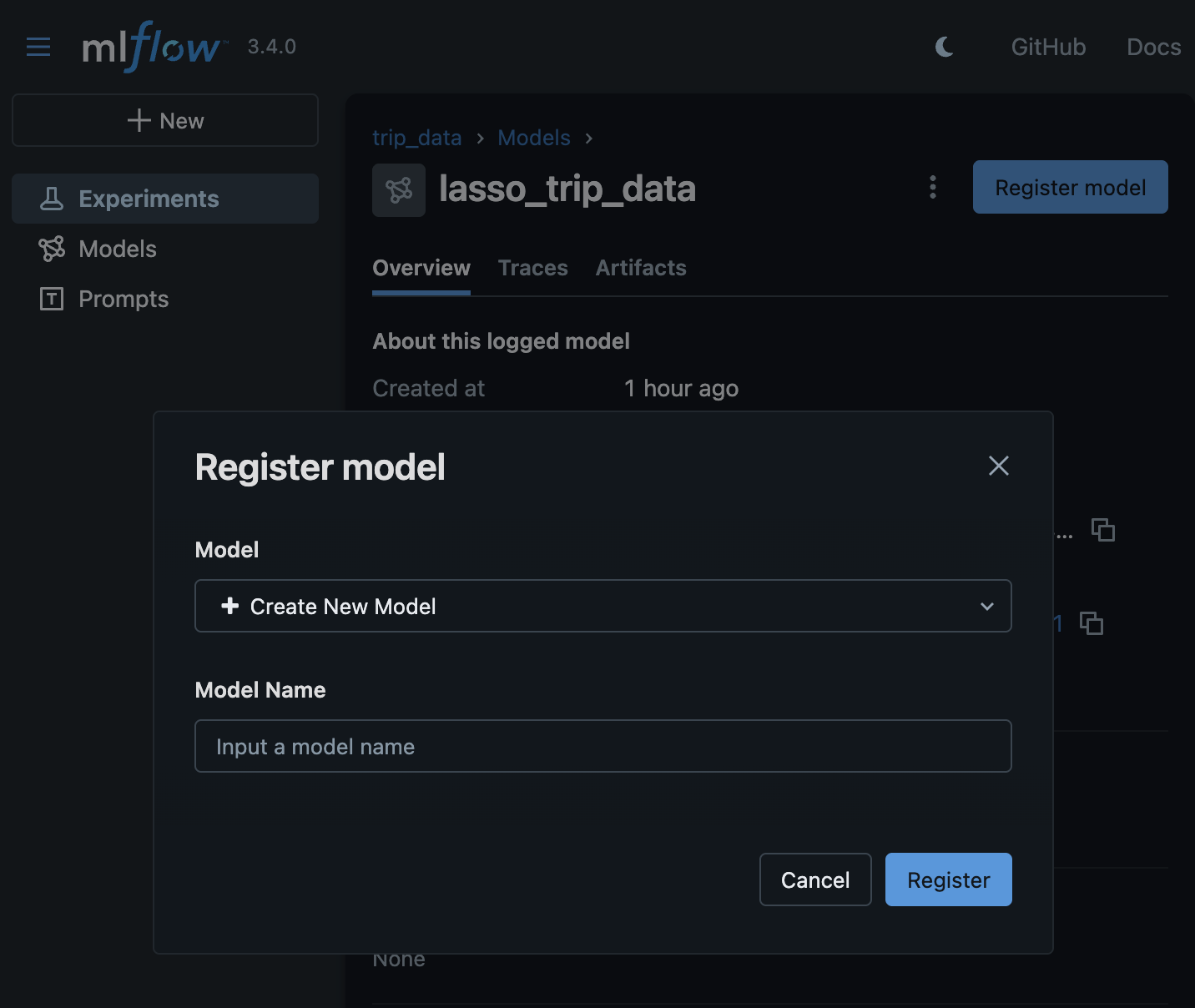
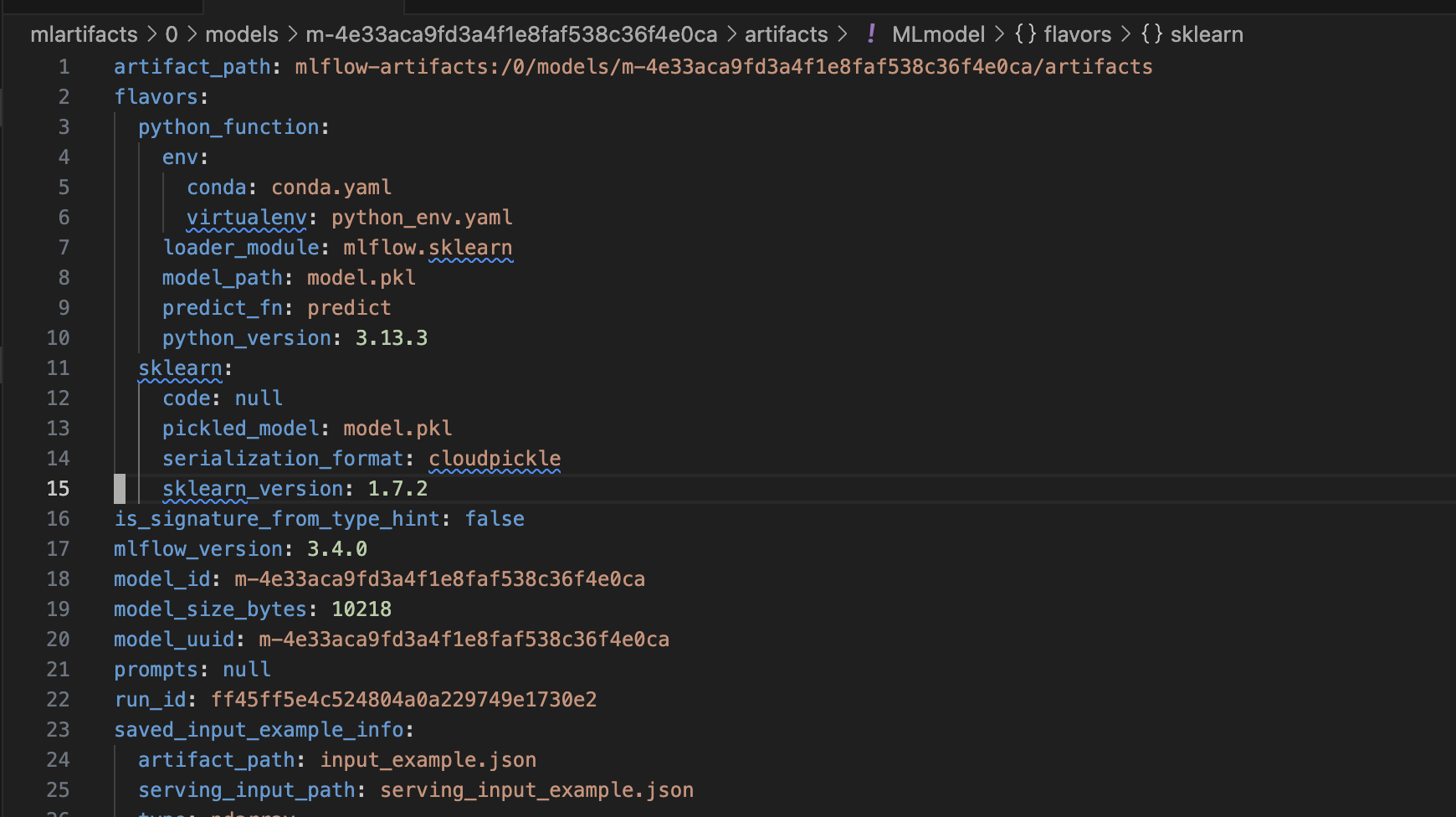
we can “log” and “register” the model with mlflow’s model registry as follows. note how we also log the signature of the model -

signature = infer_signature(X_train, lr.predict(X_train))

model_info = mlflow.sklearn.log_model(
    sk_model=lr,
    name="iris_model",
    signature=signature,
    input_example=X_train,
    registered_model_name="tracking-quickstart",
)

we can tag the model as follows for easy retrieval later

mlflow.set_logged_model_tags(
    model_info.model_id, {"Training Info": "Basic LR model for iris data"}
)

now, we can load the model as a python function and use it for inference as follows -

loaded_model = mlflow.pyfunc.load_model(model_info.model_uri)
predictions = loaded_model.predict(X_test)

Auto Logging

if we add the line mlflow.autolog() before our training code, we would not have to add the explicit log statements like above
it will automatically log the following things -
- metrics - set of metrics based on the model and library we use
- hyper params - hyper params specified for the training, plus defaults if not explicitly set
- model signature - describes input and output schema of the model
- artifacts
- dataset - used for training
we can customize its behavior like adding tags as follows -
```
mlflow.autolog(
  extra_tags={"YOUR_TAG": "VALUE"},
)
```
for GridSearchCV (helps find the best hyper parameters), it will create “parent” and “nested child” “runs”

Tracking Server

we can host the tracking server which can help with “collaboration” across teams, “audit”, etc
we can set the tracking server endpoint using MLFLOW_TRACKING_URI or mlflow.set_tracking_uri()
by default, the “metadata” is logged to the local filesystem under ./mlruns. we can configure the “backend store” as follows -
```
mlflow server --backend-store-uri sqlite:///my.db
```
i believe it uses sql alchemy underneath, so postgres, mysql, mssql, etc are supported as well
we might have to run schema migrations using mlflow db upgrade [db_uri], refer documentation for such convoluted use cases
“backend store” - where metadata like parameters, metrics and tags are stored
by default, the tracking server stores its artifacts under ./mlartifacts. we can configure the “artifact store” as follows -
```
mlflow server --artifacts-destination s3://my-bucket
```
“artifact store” - mlflow uses it to store large artifacts, e.g. model weights, images, etc
e.g. for using s3, remember to set AWS_ACCESS_KEY_ID and AWS_SECRET_ACCESS_KEY, or configure ~/.aws/credentials
our mlflow client uses paths like this - mlflow-artifacts:/, and the tracking server will automatically resolve it to the configured artifact store, e.g. s3://my-root-bucket/mlartifacts
it also supports features like multi part uploads, refer documentation for all options
there is another mode supported by tracking server, where it is not used as a proxy for the artifact store -
```
mlflow server --no-serve-artifacts --default-artifact-root s3://my-bucket
```
in this mode, the client makes requests to the tracking server to get the entire uri of the artifact store, but then interacts with the artifact store directly. pro - avoid overhead of proxying through the tracking server. con - not good from security / governance perspective
the tracking server comes with a built in “security middleware” which protects against common vulnerabilities, e.g. cors to control which web applications can access our apis
```
mlflow server --cors-allowed-origins "https://app.company.com"
```
if the server takes long to respond, e.g. when uploading or downloading large artifacts, we can set the following -
```
mlflow server --uvicorn-opts "--timeout-keep-alive=120" ...
```

Advanced Use Cases

the current experiment can also be set using MLFLOW_EXPERIMENT_NAME

we can organize experiments using “hyperparameter sweeps” / “cross validation” like so -

with mlflow.start_run(run_name="hyperparameter_sweep") as parent_run:
  mlflow.log_param("search_strategy", "random")

  for lr in [0.001, 0.01, 0.1]:
    for batch_size in [16, 32, 64]:
      with mlflow.start_run(nested=True, run_name=f"lr_{lr}_bs_{batch_size}"):
        mlflow.log_params({"learning_rate": lr, "batch_size": batch_size})
        # ... train the model etc ...

the above method can also be combined with multithreading etc, and mlflow should just work
for the best of both worlds, we can combine manual tracking with auto logging, example
we can add tags like team name, environment, etc for effective filtering and searching later, docs

Models

“mlflow models” can be used for batch inference on apache spark, realtime serving using rest api, etc
it contains an MLmodel yaml file, which is basically a config file. it defines for e.g. the different flavors of the model, e.g. pickle in case of scikit learn etc
because of these “flavors”, we can save / load the model using different formats like the scikit learn Pipeline object, a python object, etc. this in turn enables us to use it with different tools like sagemaker
for environment recreation using condas, pipenv, etc, files like requirements.txt, conda.yaml, are logged
“model signature” - defines the schema for model inputs and outputs, which helps during inference
“model input example” - provides a concrete instance of valid model input. “model signature” can be inferred if “model input example” is provided. it also generates a model serving payload example at serving_input_example.json
my understanding - typically, we call methods like save_model, log_model, load_model, etc, which mlflow already implements for common libraries like scikit learn. however for custom use cases, we can extend mlflow.models.Model, and implement its methods -
- save - save the model to a local directory
- log - log the model as an artifact
- load - load the model
my understanding - mlflow calls the interface python_function or pyfunc. this way, irrespective of the framework, or even for custom models, we define how to log and load models
we can use mlflow.models.predict to test our models in a virtual, isolated environment. it helps validate if the dependencies logged with the model are correct / enough, we can use it to validate with some sample input data i.e. if it interacts with the model as expected, etc. it supports uv as well

Models from Code

“models from code” - define and log models from standalone python scripts
useful when we want to log models that can be stored as a code representation
they do need to use optimized weights through training, and so they do not need to use pickle etc
they can for instance rely on external services, e.g. langchain chains
refer documentation for more details

Evaluation

mlflow supports this feature for both classification and regression
what metrics it calculates automatically can be found in the documentation here, e.g. “performance metrics” (e.g. roc / auc, f1 score, etc), “visualizations” (e.g. confusion matrix, precision recall curve, etc)
it also supports “feature importance” via “shap”
“shap” or “shapely adaptive explanations” helps us understand what drives our model’s predictions. they are required when the models are complex, in cases like healthcare / finance where interpretability is crucial, etc
e.g. to enable shap logging, we add evaluator_config={"log_explainer": True}
lot of functionality and examples can be found in documentation around how to log custom metrics, how to define some thresholds for the models to pass, how to run evaluation in batches for large datasets, how to configure shap, etc

signature = infer_signature(X_test, model.predict(X_test))
model_info = mlflow.sklearn.log_model(model, name="model", signature=signature)

result = mlflow.models.evaluate(
  model_info.model_uri,
  eval_data,
  targets="label",
  model_type="classifier",
  evaluators=["default"],
)

print(f"Accuracy: {result.metrics['accuracy_score']:.3f}")
print(f"F1 Score: {result.metrics['f1_score']:.3f}")
print(f"ROC AUC: {result.metrics['roc_auc']:.3f}")

Serving

mlflow allows deploying models to various “targets” like local environments, cloud environments like aws / azure, kubernetes, etc
it already helps package models and their dependencies using virtual environments, docker images, etc
it also helps launch an inference server with rest endpoints using frameworks like fast api

we can run “batch inference” as follows -

mlflow models predict -m models:/<model_id> -i input.csv -o output.csv

or using python

import mlflow

model = mlflow.pyfunc.load_model("models:/<model_id>")
predictions = model.predict(pd.read_csv("input.csv"))
predictions.to_csv("output.csv")

Machine Learning

Supervised Machine Learning

CRISP DM

Model Selection

Regression

Classification

Evaluation

Cross Validation

Deployment

Decision Trees

Random Forest

Gradient Boosting

MLOps Introduction

Experiment Tracking

Deployment

Tracking

Basics

Auto Logging

Tracking Server

Advanced Use Cases

Models

Models from Code

Evaluation

Serving

Further Reading

High Level Design IV

Indian History

High Level Design III